


Abstract
We present results from two long-duration general relativistic magneto-hydrodynamic (GRMHD) simulations of advection-dominated accretion around a non-spinning black hole. The first simulation was designed to avoid significant accumulation of magnetic flux around the black hole. This simulation was run for a time of 200 000 GM/c3 and achieved inflow equilibrium out to a radius ∼90 GM/c2. Even at this relatively large radius, the mass outflow rate  is found to be only 60 per cent of the net mass inflow rate
  into the black hole. The second simulation was designed to achieve substantial magnetic flux accumulation around the black hole in a magnetically arrested disc. This simulation was run for a shorter time of 100 000 GM/c3. Nevertheless, because the mean radial velocity was several times larger than in the first simulation, it reached inflow equilibrium out to a radius ∼170 GM/c2. Here,
  becomes equal to
  . Since the mass outflow rates in the two simulations do not show robust convergence with time, it is likely that the true outflow rates are lower than our estimates. The effect of black hole spin on mass outflow remains to be explored. Neither simulation shows strong evidence for convection, though a complete analysis including the effect of magnetic fields is left for the future.
1 Introduction
Black hole (BH) accretion occurs via at least two distinct modes: (1) a standard thin accretion disc (Shakura & Sunyaev 1973; Novikov & Thorne 1973; Frank, King & Raine 2002), and (2) an advection-dominated accretion flow (ADAF; Narayan & Yi 1994, 1995b; Abramowicz et al. 1995; Ichimaru 1977; see Narayan, Mahadevan & Quataert 1998; Frank et al. 2002; Kato, Fukue & Mineshige 2008; Narayan & McClintock 2008 for reviews). Thin discs are present around stellar-mass and supermassive BHs that accrete at a substantial fraction ∼ a few to 100 per cent of the Eddington rate, while ADAFs are typically found at lower accretion rates  .1
.1
The accreting gas in an ADAF is radiatively inefficient; hence an ADAF is also referred to as a radiatively inefficient accretion flow (RIAF). The low radiative efficiency, on top of the already low accretion rate, makes ADAFs highly underluminous and difficult to observe. On the other hand, the vast majority of both stellar-mass and supermassive BHs in the Universe are in the ADAF state, a notable example being Sgr A*, the supermassive BH at the centre of our own Galaxy (Narayan, Yi & Mahadevan 1995; Yuan, Quataert & Narayan 2003).
A simple one-dimensional model of gas dynamics in an ADAF (Narayan & Yi 1994) reveals two interesting complications. First, the Bernoulli parameter of the gas tends to be positive. This means that the gas is not gravitationally bound to the BH, or at best is only weakly bound. Therefore, an ADAF is likely to have powerful jets and mass outflows, as recognized in the very first papers (Narayan & Yi 1994, 1995a). The connection between ADAFs and relativistic jets has become increasingly clear over the years (e.g. Narayan & McClintock 2008 and references therein). However, it is presently unknown whether or not ADAFs have quasi- or non-relativistic winds, and if so how much mass they lose via these winds.
Some authors (e.g. Blandford & Begelman 1999; Begelman 2012) have suggested that winds in ADAFs are so powerful that the mass accretion rate  on the BH is as much as ∼5 orders of magnitude less than the mass supply rate
  at the outer edge of the accretion flow, say at the Bondi radius. In effect, these authors took the Bernoulli argument for strong outflows proposed in the original ADAF papers (Narayan & Yi 1994, 1995a), and postulated that ADAFs would have not just strong outflows, but overwhelmingly strong outflows. Other authors (Ogilvie 1999; Abramowicz, Lasota & Igumenshchev 2000), however, argued that the Bernoulli parameter is not a good diagnostic for mass loss, especially in the case of viscous non-steady flows.
Yuan et al. (2003) attempted to constrain the mass loss in Sgr A* using radio data on Faraday rotation (Agol 2000; Aitken et al. 2000; Quataert & Gruzinov 2000a; Bower et al. 2003; Marrone et al. 2007). They concluded that, for this source, the decrease of  between the Bondi radius and the BH is of the order of one to two orders of magnitude. More recently, a few studies (e.g. Allen et al. 2006; McNamara, Rohanizadegan & Nulsen 2011) have shown that many radio-loud active galactic nuclei require a power source comparable to or even greater than what Bondi accretion can supply. Even if the power source of the jet is BH spin energy, one still requires a significant mass accretion rate on to the BH to tap this spin power (Narayan & Fabian 2011; Tchekhovskoy, Narayan & McKinney 2011). Therefore, in the above radio sources, there cannot be significant mass loss between the Bondi radius and the BH horizon.
The second potential complication in the dynamics of ADAFs is that the entropy gradient is large and highly unstable according to the Schwarzschild criterion (Narayan & Yi 1994). One might thus suspect that ADAFs will be very convective. On the other hand, the angular momentum profile has a stable gradient. It is thus not clear whether the flow is ultimately stable or unstable to convection. Analytical models of convection-dominated accretion flows (CDAFs; Narayan, Igumenshchev & Abramowicz 2000; Quataert & Gruzinov 2000b) have been developed, but their relevance to real ADAFs is unclear (see Narayan et al. 2002; Balbus & Hawley 2002 for conflicting views).
Both mass-loss and convection involve multi-dimensional flows, which are best studied via numerical simulations. In addition, since the ‘viscosity’ that drives accretion originates in the magnetorotational instability (MRI; Balbus & Hawley 1991, 1998), magnetic fields play a critical role. This makes analytical studies even less tractable. Fortunately, multi-dimensional numerical magneto-hydrodynamic (MHD) simulations are now feasible. Indeed, the limit of a non-radiative ADAF is relatively easy to simulate, since there is no radiation physics involved. Moreover, ADAFs are geometrically thick and are less demanding in terms of spatial resolution. We briefly review here the large literature on ADAF simulations.
Early numerical simulations of ADAFs employed pseudo-Newtonian codes with purely hydrodynamic viscosity. Pioneering work by Stone, Pringle & Begelman (1999) indicated that such flows are convective and that a significant fraction of the inflowing mass near the equatorial plane flows out along the poles in a strong outflow. Similar results, viz., convection, equatorial inflow and bipolar outflow, were obtained also by Igumenshchev & Abramowicz (1999, 2000). In the latter paper, the authors found that bipolar outflows required high values of the viscosity parameter α, while low-viscosity models exhibited weaker outflows but had strong convection. Very recently, Yuan, Wu & Bu (2012b, see also Yuan, Bu & Wu 2012a) have carried out 2D hydrodynamic simulations of ADAFs which cover a very large range of radius and show fairly strong outflows. Most of the outflowing gas is bound to the BH in the sense that it has a negative Bernoulli parameter, yet it reaches the outer boundary of the simulation without turning around. Li, Ostriker & Sunyaev (2012) have carried out hydrodynamic simulations of ADAFs including the effects of bremsstrahlung cooling and electron thermal conduction.
Although interesting, hydrodynamic α-viscosity simulations are ultimately not realistic since accretion flows have magnetic fields and MRI-driven turbulence. It is thus necessary to include magnetic fields consistently. Pseudo-Newtonian MHD simulations have been performed by a number of authors. Machida, Hayashi & Matsumoto (2000) and Machida, Matsumoto & Mineshige (2001) observed temporary outflows of mass in their MHD simulations and showed that substantial accretion energy can be released in the vicinity of the BH via magnetic reconnection. They also claimed that the initial configuration of the magnetic field may play an important role in determining the mass outflow rate. Using axisymmetric (2D) models, Stone & Pringle (2001) showed that significant outflows originate at radii beyond r ∼ 10 (we express lengths in BH mass units: GM/c2). Similarly, Hawley & Balbus (2002) observed outflows for all radii outside the innermost stable circular orbit (ISCO), though they used a definition of inflow and outflow based on cyclindrical coordinates (all other authors use spherical coordinates) which makes their outflow estimates somewhat ambiguous.
Convective motions were evident in MHD simulations performed by Machida et al. (2001), indicating, according to the authors, that convection is a rather general phenomenon in RIAFs. On the other hand, Stone & Pringle (2001) concluded that the turbulence seen in their MHD simulations was driven by the MRI, not convection. Similarly, Hawley & Balbus (2002) noted that, although their models were unstable according to the classical Hoiland criteria, the flows appeared not to be convective. On the other hand, a simulation by Igumenshchev, Narayan & Abramowicz (2003), which was initialized with purely toroidal magnetic field, showed significant convection, and appeared to be similar to a CDAF. The same authors found that, if they initialized the simulation with a poloidal magnetic field, the disc structure was completely different from the toroidal case. The poloidal case led to a configuration in which the magnetic field strongly resisted the accreting gas, leading to what the authors later called a ‘magnetically arrested disc’ (MAD; Narayan, Igumenshchev & Abramowicz 2003). In a series of numerical MHD simulations, Pen, Matzner & Wong (2003) and Pang et al. (2011) found little evidence for either outflows or convection. Even though the entropy gradient was unstable the gas was apparently prevented from becoming convective by the magnetic field. They coined the term ‘frustrated convection’ to describe this behaviour.
Beginning with the work of De Villiers, Hawley & Krolik (2003), accretion flows have been studied using general relativistic magneto-hydrodynamic (GRMHD) codes. De Villiers et al. (2003) observed two kinds of outflows: bipolar unbound jets and bound coronal flow. The coronal flow supplied gas and magnetic field to the coronal envelope, but apparently did not have sufficient energy to escape to infinity. The jets on the other hand were relativistic and escaped easily, though carrying very little mass. Jets have been studied in detail by a number of authors (McKinney & Gammie 2004; De Villiers et al. 2005; McKinney 2006). Beckwith, Hawley & Krolik (2008, 2009) and McKinney & Blandford (2009) noted that the power emerging in the jets depended strongly on the assumed magnetic field configuration. While dipolar fields produced strong jets, a quadrupolar field led to only weak, turbulent outflows.
Tchekhovskoy et al. (2011) simulated a MAD system around a rapidly spinning BH, and obtained very powerful jets with energy efficiency η > 100 per cent, i.e. jet power greater than 100 per cent of  , where
  is the mass accretion rate on to the BH. Their work showed beyond doubt that at least some part of the jet power had to be extracted from the spin energy of the BH. The jet–spin connection for MAD systems has been explored in greater detail by McKinney, Tchekhovskoy & Blandford (2012). These authors coined the term ‘magnetically choked accretion flow’ (MCAF) to describe the MAD configuration.
Returning to the present paper, the goal here is to use GRMHD simulations of ADAFs around BHs to investigate the importance of mass outflows, and if possible convection. Our simulations are run for a longer duration than most previous work. The questions we address require us to analyse the properties of the accretion flow over as wide a range of radius as possible. The only way to obtain converged results over such large volumes is by running simulations for a very long time. We introduce a new measure of convergence, or more accurately a test of internal consistency. As per this criterion, our simulations give converged time-steady flows over a range of up to 100 in radius. This turns out to be still not as large as we would like. Nevertheless, it permits us to reach some interesting conclusions.
Within the realm of ADAFs, we expect answers to depend on several factors. One important factor has already been mentioned, viz., the magnetic field topology in the accreting gas. The role of field topology for mass outflows (as distinct from relativistic jets) has been largely unexplored. The recent work of McKinney et al. (2012) is one of the first studies in this area.
In this paper we consider two distinct magnetic topologies and describe one long-duration simulation for each topology. In one simulation, we carefully arrange the initial seed magnetic field (which is later amplified via the MRI) such that the accreting gas does not become magnetically arrested despite the long duration of the simulation. We call this the ADAF/SANE simulation (where SANE stands for ‘standard and normal evolution’). In the second simulation, we set up the magnetic field topology such that the accretion flow very quickly becomes magnetically arrested and then remains in this state for the duration of the run. We call this the ADAF/MAD simulation (where, as stated earlier, MAD stands for ‘magnetically arrested disc’).
A second obvious parameter that will affect the properties of an ADAF is the spin of the central BH. Numerical studies of jets, for instance, clearly show that jet power correlates strongly with BH spin (McKinney 2006; Tchekhovskoy et al. 2011; Tchekhovskoy & McKinney 2012; Tchekhovskoy, McKinney & Narayan 2012). Observationally too, there is evidence for such a correlation (Narayan & McClintock 2012). In this paper we focus on the case of a non-spinning BH: a* ≡ a/M = 0. We view such a system as the purest form of an ADAF, where the only available energy source is gravitational potential energy released via accretion. By simulating an ADAF around a non-spinning BH using a GRMHD code, we can more easily relate our results to analytical studies as well as previous non-relativistic simulations. In the future we plan to run long-duration GRMHD simulations of ADAFs around spinning BHs. Those simulations will have two sources of energy, accretion and BH spin. By comparing them with the simulations described here we should be able to evaluate the role of BH spin.
The plan of the paper is as follows. In Section 2, we briefly describe the simulation methods we employ, which are similar to those we have used in previous work. In Section 3, we discuss in detail our results from the ADAF/SANE and ADAF/MAD simulations, focusing in particular on mass outflows. In Section 4, we bring together the results of the previous sections and try to assess the nature of the accretion flow in the two simulations. In Section 5, we conclude with a discussion.
2 Details of the Simulations
2.1 Computation method
The simulations described here were done with the 3D GRMHD code harm (Gammie, McKinney & Tóth 2003; McKinney 2006; McKinney & Blandford 2009), which solves the ideal MHD equations of motion of magnetized gas in the fixed general relativistic metric of a stationary BH. The equation of state of the gas is taken to be u = p/(Γ − 1), where u and p are the internal energy and pressure, and Γ is the adiabatic index. The code conserves energy to machine precision, hence any energy lost at the grid scale, e.g. through turbulent dissipation or numerical reconnection, is returned as entropy of the gas. There is no radiative cooling. The code works in dimensionless units where GM = c = 1. Thus, all lengths and times in this paper are given in units of GM/c2 and GM/c3, respectively.
A key feature of our simulations is the extremely long run time: 200 000 time units for the ADAF/SANE simulation, and 100 000 time units for the ADAF/MAD simulation. To avoid spurious signals reaching the region of interest from the boundary of the simulation, our grid extends out to a very large radius, ∼105. At the same time, we require good resolution in the inner regions in order to study the structure of the flow. To satisfy both requirements, we use a grid with 256 cells in the radial direction, where the cells are distributed uniformly in log r at smaller radii and spaced hyper-logarithmically near the outermost radii.
In the θ direction, we employ 128 cells, distributed non-uniformly so as to provide adequate resolution both in the geometrically thick equatorial region, where the bulk of the gas accretes, and in the polar region, where a relativistic jet might flow out. In order to follow such a jet as it collimates at large distance, we use the grid developed by Tchekhovskoy et al. (2011) in which the θ resolution near the pole increases with increasing radius (see Fig. 1).2
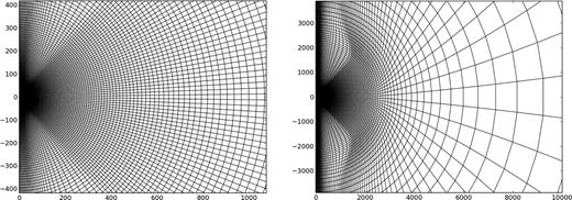
Poloidal plane of the grid used in the simulations, shown at two zoom levels.
Finally, we use a uniform grid of 64 cells in the azimuthal direction, covering the full range of φ from 0 to 2π.
2.2 Initial conditions
The fluid initially rotates around the BH in a torus in hydrostatic equilibrium: a ‘Polish doughnut’ (Kozlowski, Jaroszynski & Abramowicz 1978). The ADAF/SANE and ADAF/MAD simulations begin with the same torus. It has inner edge at rin = 10 and extends to r ∼ 1000 (Fig. 2 and 3). The angular momentum of the torus is constant inside rbreak = 42. Outside rbreak, the angular momentum is 71 per cent of the Keplerian value and is constant on von Zeipel cylinders. The entropy is constant everywhere,  , and the Bernoulli is small and negative, −Be ∼ 10−2 to 10−3 (in units of c2). The torus is described in detail in Penna, Kulkarni & Narayan (2012).
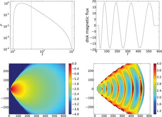
Initial configuration of the ADAF/SANE simulation. The top two panels show the mid-plane density and the magnetic flux threading the equatorial plane as a function of radius. Note the extended size of the initial torus, which is required for the extremely long duration of this simulation. Note also the multiple oscillations in the magnetic flux, which prevents the accreting gas from reaching the MAD state. The lower two panels show the logarithm of the density ρ and the gas-to-magnetic pressure ratio β of the initial torus in the poloidal plane.
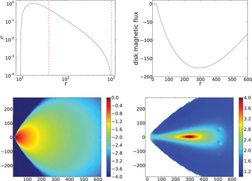
Similar to Fig. 2 but for the ADAF/MAD simulation. The main difference is that the torus here has a single loop of field centred at radius r = 300. As a result, accretion causes magnetic flux of one sign to accumulate around the BH, leading to the MAD state.
The initial magnetic field is purely poloidal. The magnetic field in the case of the ADAF/SANE simulation is broken into eight poloidal loops of alternating polarity (Fig. 2). Each loop carries the same amount of magnetic flux, so the BH is unable to acquire a large net flux over the course of the simulation. The normalization of the magnetic field is adjusted such that the gas-to-magnetic pressure ratio, β, in the equatorial plane has a minimum value ∼100 for each of the eight loops. Instead of using multiple poloidal loops, another way of setting up an ADAF/SANE simulation is to use a toroidal initial field (e.g. Model A in Igumenshchev et al. 2003 and Model A0.0BtN10 in McKinney et al. 2012).
The initial magnetic field of the ADAF/MAD simulation forms a single poloidal loop centred at r = 300 (Fig. 3). The gas accreted by the BH in this simulation has the same orientation of the poloidal magnetic field throughout the run, so the net flux around the BH increases rapidly and remains at a high value. The accretion flow is thus maintained in the MAD state. The minimum value of β in the initial torus is ∼50.
The magnetic field construction is described in detail in Penna et al. (2012).3
2.3 Preliminary discussion of the simulations
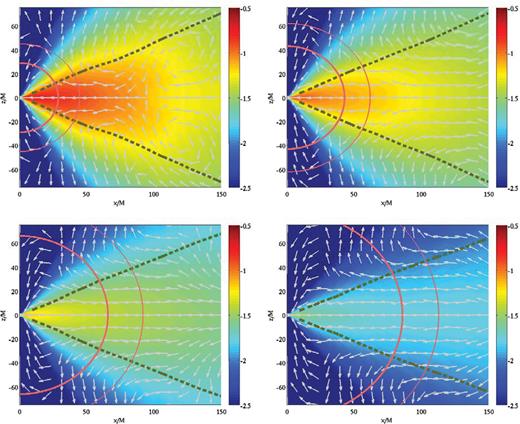
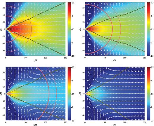
The two panels in Fig. 4 show snapshots from the end of the ADAF/SANE and ADAF/MAD simulations. In each panel, the black and white streaks and red arrows show velocity streamlines in the poloidal plane at azimuthal angle φ = 0, and the dashed lines correspond to one density scale height. The main difference between the two simulations is that the SANE run exhibits more turbulence compared to the MAD run.
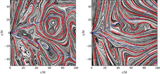
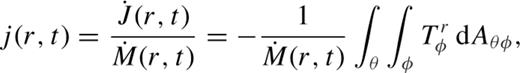
Left: snapshot of the ADAF/SANE simulation at t = 200 000. Black and white streaks as well as red arrows represent flow streamlines. Note the turbulent eddies. The blue dashed lines indicate the density scale height. Right: snapshot of the ADAF/MAD simulation at t = 100 000M. There is much less turbulence.
 , the accreted specific energy e and the accreted specific angular momentum j, at radius r and time t, as follows:
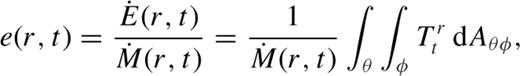
 is an area element in the θ–φ plane, ρ is rest mass density, uμ is the four-velocity, and
  and
and  are components of the stress-energy tensor describing the radial flux of energy and angular momentum, respectively:

 ,
,  ,
,  are positive when the corresponding fluxes are pointed inwards. More useful than e is the quantity (1 − e), which is the ‘binding energy’ of the accreting gas relative to infinity.
Fig. 5 shows the time evolution of  , j, (1 − e) and φBH as a function of time for the ADAF/SANE and ADAF/MAD simulations. The first three quantities are measured at r = 10,4 while the fourth is (by definition) evaluated at the horizon r = rH. We see that the magnetization parameter φBH behaves very differently in the two simulations. In the ADAF/SANE simulation, φBH remains small, except for one spike at time t ∼ 140 000. In contrast, in the ADAF/MAD simulation, the magnetization quickly rises to a value ∼50 and remains at this high value for the rest of the run. As explained in Tchekhovskoy et al. (2011), the plateau in φBH corresponds to the MAD state where the BH has accepted as much magnetic flux as it can hold for the given mass accretion rate. Any additional flux brought in by the accreting gas remains outside the horizon, where it ‘arrests’ the accretion flow.
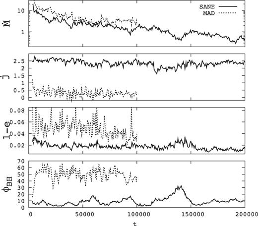
Variations of  , j and (1 − e) at r = 10, and φBH at r = rH, as a function of time. Solid lines correspond to the ADAF/SANE simulation and dotted lines to the ADAF/MAD simulation. Note the very different behaviours of the two simulations. The decrease of
  with increasing time is explained in Fig. 6 and the text.
Corresponding to the dramatic difference in φBH in the two simulations, there are related differences in both the binding energy flux (1 − e) and the specific angular momentum flux j. The quantity (1 − e) is about two to three times larger in the MAD simulation, which indicates that the MAD system has more energy flowing out to infinity compared to the SANE simulation. Coincident with the spike in φBH in the ADAF/SANE simulation at t ∼ 140 000, there is a corresponding spike in (1 − e). During this period, the SANE simulation seems to have made a brief detour close to the MAD limit.
The specific angular momentum flux j is about an order of magnitude less in the MAD simulation compared to the SANE simulation. Once the gas has attained the MAD state, it transfers very little angular momentum to the BH. Instead, angular momentum is transported out, largely through the magnetic field. This implies that an ADAF/MAD accretion flow will cause little spin-up of the BH. Indeed, as Tchekhovskoy et al. (2012) and McKinney et al. (2012) have shown, if the BH has virtually any non-zero value of a*, an ADAF/MAD flow will cause spin-down rather than spin-up.
Before discussing the behaviour of  in Fig. 5, we first describe the method we use in the rest of the paper to analyse the time evolution of quantities. We divide the data from each simulation into a number of ‘time chunks’ which are logarithmically spaced in time. In the case of the ADAF/SANE simulation we have six time chunks, S1–S6, with each successive chunk being twice as long as the previous one (Table 1). This logarithmic spacing is well-suited for the issues discussed in this paper since most of the quantities we are interested in show power-law behaviour as a function of both time and radius. In the case of the shorter ADAF/MAD simulation we divide the data into five time chunks, M1–M5 (Table 2). Note that there is no overlap between chunks, and hence each chunk provides independent information.
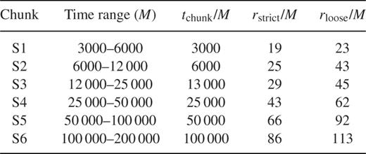
Time chunks in the ADAF/SANE simulation.
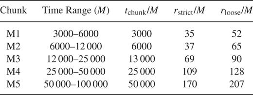
Time chunks in the ADAF/MAD simulation.
Returning to Fig. 5, we see that  shows a large decrease with time in both simulations. Fig. 6 explains the reason for this. Since the accreting gas originates in the initial gas torus shown in Fig. 2 and 3, the mass distribution in the flow has to match smoothly to this mass reservoir. With increasing time, the radius range over which the flow achieves steady state increases (as discussed in greater detail in the following sections). At the boundary of the steady-state region, quantities like the surface density, Σ = (1/2π)∫∫ρ dAθφ (shown in Fig. 6), have to match the corresponding values in the torus, and this fixes
  for that epoch. Since the torus has a prescribed variation of Σ with r, we thus have a pre-determined variation of
  with time. In hindsight, it might have been better to design the initial torus so as to obtain a roughly constant
  with time. An alternate approach, pioneered by Igumenshchev et al. (2003), is to inject mass steadily at some outer radius rather than to start with a fixed total mass in a torus.
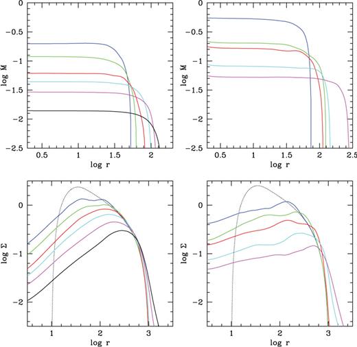
Top left: the variation of the mean mass accretion rate  versus r in the ADAF/SANE simulation for the six independent time chunks S1–S6. The colour code is as follows: S1 (blue), S2 (green), S3 (red), S4 (cyan), S5 (magenta), S6 (black). The flat region of each curve identifies the range of r over which the accreting gas is in inflow equilibrium. This range increases monotonically with time, as one expects. Top right: similar plot for the ADAF/MAD simulation for the five time chunks M1–M5. Colour code: M1 (blue), M2 (green), M3 (red), M4 (cyan), M5 (magenta). Bottom left: an explanation for why the mass accretion rate shown in Fig. 5 declines secularly with time in the ADAF/SANE simulation. In each time chunk, the surface density Σ has to match smoothly to the Σ profile of the initial torus (dotted curve). Therefore, the decrease in
  is purely a consequence of the initial conditions. Bottom right: similar plot for the ADAF/MAD simulation.
2.4 Resolving the MRI
 ,
,  , and the magnetic field components,
  ,
,  , are evaluated in the orthonormal fluid frame. The fluid's angular velocity is Ω. The parameter
  is defined such that it becomes
  in the limit of a vertical field, where λMRI is the wavelength of the fastest growing mode of the linear MRI.
Hawley et al. (2011) considered a number of diagnostics, principally  and dimensionless viscosity parameter α, but also
  and plasma β ≡ Pgas/Pmag, as a function of numerical resolution. They studied both local shearing boxes and global Newtonian discs and concluded that simulations with
  and
and  are sufficiently well resolved to give quantitatively converged results. They also state that simulations with smaller values of
  , but correspondingly larger values of
  , are equally good. Thus, we write their criterion for convergence as
  . In addition, they recommend that the ratio
  near the disc mid-plane should be no larger than 4.
In related work, Sorathia et al. (2012) simulated global (but unstratified) Newtonian discs using a wide range of resolutions and showed that the magnetic tilt angle, which is related to the ratio  mentioned above, is a good diagnostic for evaluating convergence. On the basis of this diagnostic, they suggest that a ratio
  is sufficient for convergence, but a ratio of 4 tends to be somewhat under-resolved (see their fig. 11c). Thus, their criterion is stricter than the one proposed by Hawley et al. (2011).
Our simulations have  10–20 throughout the initial magnetic loops. The initial
  is zero because the loops are poloidal. For the ADAF/SANE run, the fluid inside r = 100 and within one density scale height of the mid-plane has
  and
and  between 10 and 20, i.e.
  , which is sufficient according to Hawley et al. (2011). Our numerical grid has
  at the mid-plane, which is safe according to Hawley et al. (2011) and borderline according to Sorathia et al. (2012). Overall, we conclude that our ADAF/SANE simulation is adequately resolved. Our ADAF/MAD simulation has
  and
and  , so this simulation is very well resolved.
Exploring the issue of convergence further, we note that the grid used in the present study is very similar to the one employed by Tchekhovskoy et al. (2011) for simulating their MAD models. These authors tested convergence by increasing the number of cells in the φ direction by a factor of 2, i.e. using 128 cells over the range φ = 0–2π instead of the fiducial 64 cells. The results they obtained with this increased resolution agreed with those from their fiducial runs, indicating that 64 cells over 2π in φ (or 32 cells over a wedge of angle π) are sufficient for convergence. Thus we are confident that our ADAF/MAD run has sufficient resolution.
McKinney et al. (2012) describe a large number of simulations, of which one sequence of models, A*BtN10, was initialized with a purely toroidal field. These models, which evolve into configurations similar to our ADAF/SANE simulation, used a resolution of Nr = 128, Nθ = 64, Nφ = 128, which is slightly different from, but generally similar to, our resolution, Nr = 256, Nθ = 128, Nφ = 64. In addition, McKinney et al. (2012) considered one high-resolution toroidal-field model, A0.94BtN10HR, with Nr = 256, Nθ = 128, Nφ = 256. Looking at the detailed results, it is not obvious that their high-resolution model is distinctly superior to their standard lower-resolution models.
Based on all of the above, we believe the two simulations described in this paper are adequately resolved.
3 Analysis and Results
3.1 Criteria for convergence and steady state
Fig. 7 shows time-averaged, φ-averaged, z-symmetrized results for the final four time chunks, S3, S4, S5, S6, of the ADAF/SANE simulation. The strong averaging of the simulation data eliminates most of the turbulent fluctuations that were evident in Fig. 4, and enables us to focus on mean properties of the flow. The accretion flow is geometrically thick, as expected, and the gas velocity is predominantly inwards within one scale height of the mid-plane. At higher latitudes, many velocity arrows point away from the BH, indicating that there is mass outflow. At yet higher latitudes, as we approach the poles, the gas appears again to flow in towards the BH. It is therefore not obvious how much gas actually flows out to infinity. We discuss this question in detail in the next subsection.
Average flow properties of the ADAF/SANE simulation during chunks S3 (top left), S4 (top right), S5 (bottom left) and S6 (bottom right). In each panel, the flow has been averaged over the duration of the chunk tchunk (Table 1), over azimuthal angle φ, and symmetrized around the mid-plane. Colour indicates log ρ, arrows indicate direction (but not magnitude) of the mean velocity and slanting dashed lines indicate the local density scale height. The two circular solid lines correspond to the steady-state radius limits rstrict (thick line) and rloose (thin line), computed using the mean radial velocity within one scale height of the mid-plane (see text and Table 1 for details).
Fig. 8 shows an equivalent plot for the ADAF/MAD simulation, corresponding to the final four time chunks, M2, M3, M4, M5. Comparing Fig. 7 and 8, the flow streamlines in the MAD run show more well-organized outflow behaviour. There are also outflowing streamlines along the axis, suggesting some kind of polar jet. However, very little energy, and practically no mass, flows along this jet. Therefore, for all practical purposes, the simulation does not have a jet.


The philosophy behind the above criteria is that we expect the flow to reach inflow equilibrium on a time-scale of the order of the viscous time. Further, it takes a few viscous times to average out fluctuations. The strict criterion has ttot = 2tchunk = 4tvisc, which is a fairly safe and conservative choice, while the loose criterion takes a more optimistic view of how soon inflow equilibrium is achieved. Note that Penna et al. (2010) defined inflow equilibrium by the condition ttot = 2tvisc, which is the same as our present loose criterion. The values of tchunk, rstrict and rloose for the various time chunks are listed in Tables 1 and 2, and rstrict and rloose are shown as circular solid lines in Fig. 7 and 8. It will be noticed that the objectively determined rstrict and rloose are compatible with values one might deduce by visual inspection of Fig. 6.
In Fig. 7 and 8, the time-averaged velocity streamlines are well-behaved within the respective inflow equilibrium regions of the four panels. Note also that the steady-state zone is much more extended in the MAD simulation compared to the SANE simulation. For instance, MAD chunk M5, which has run only half as long as SANE chunk S6, is converged out to a substantially larger radius (compare the values of rstrict, rloose in Tables 1 and 2). The reason is the larger radial velocity of the gas in the MAD simulation (compare Fig. 11 and 12).
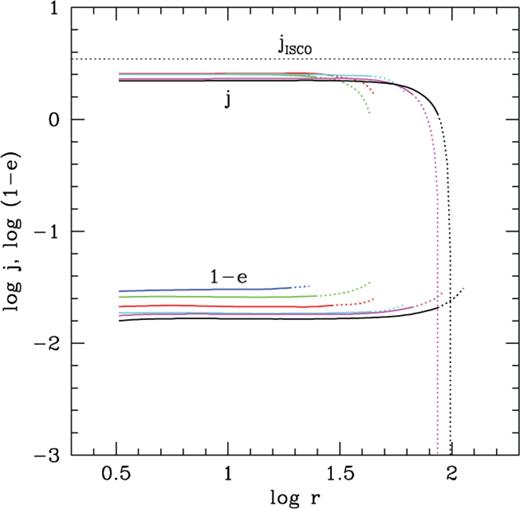
The black dotted line at the top labelled jISCO corresponds to the angular momentum of a Keplerian orbit at the radius of the ISCO. This represents the specific angular momentum flowing into the BH in the case of a standard thin disc (Novikov & Thorne 1973). The cluster of lines just below the dotted line shows the run of specific angular momentum flux with radius j(r) corresponding to chunks S1 (blue), S2 (green), S3 (red), S4 (cyan), S5 (magenta) and S6 (black) for the ADAF/SANE simulation. All of these curves lie below the NT curve, indicating that the ADAF flow is sub-Keplerian, as predicted by theory. Each of the curves has a flat segment where the time-averaged flow shows excellent steady-state convergence and a region at larger radii where j deviates from steady state. The bottom set of lines (same colour coding) shows the specific binding energy flux (1 − e) for the same time chunks. For both sets of lines, the solid and dotted line segments correspond to r ≤ rstrict and r ≤ rloose, respectively (see text and Tables 1 and 2).
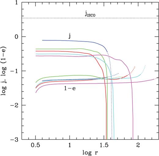
Similar to Fig. 9, but for the ADAF/MAD simulation. The colour coding is: chunk M1 (blue), M2 (green), M3 (red), M4 (cyan), M5 (magenta).
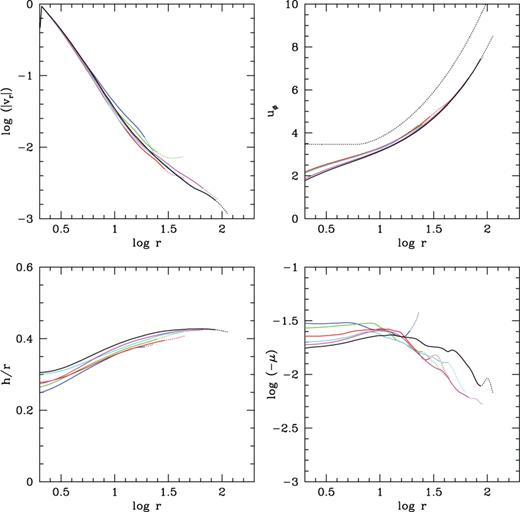
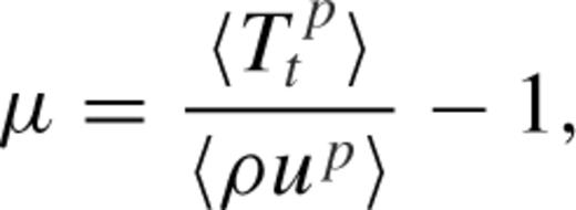
Top left: the density-weighted mean radial velocity of the gas in the ADAF/SANE simulation within one scale height of the mid-plane during time chunks S1–S6. The colour code and line types are the same as in Fig. 9. Top right: a similar plot for the density-weighted specific angular momentum uφ of the accreting gas. The black dotted line shows the Keplerian profile of angular momentum for a standard thin accretion disc (Novikov & Thorne 1973). Bottom left: plot of the density scale height h/r for the six time chunks. Bottom right: plot of the mid-plane values of μ, which represents the normalized flux of the Bernoulli parameter (see equation 13). The fact that μ is negative indicates that the mid-plane gas is bound to the BH.
When the accretion flow has reached inflow equilibrium, we expect θ- and φ-integrated fluxes of conserved quantities, as defined in equations (1)–(3), to be independent of radius. Recall that there is no radiative cooling, hence there ought to be strict conservation of not only mass, but also energy and angular momentum. As time proceeds, the range of r over which these fluxes are constant will increase, and should track rstrict or rloose (depending on the degree of constancy one requires).
Fig. 9 shows the fluxes of specific angular momentum j and specific binding energy (1 − e) for the six time chunks in the ADAF/SANE simulation. The range of radius over which these fluxes are in inflow equilibrium increases from time chunk S1 to S6, i.e. with increasing time, as expected. The solid line segments in the plot correspond to the strict criterion r ≤ rstrict, and the dotted lines correspond to the loose criterion r ≤ rloose. This convention is adopted in all later plots.
Fig. 9 highlights the difference in convergence properties between the two criteria. Although the strict criterion is not perfect, the fluxes do remain nearly constant over the radius ranges defined by this criterion. The loose criterion, however, shows unacceptably large deviations from flux constancy. Hereafter, we quote quantitative results only for regions satisfying the strict criterion (the inner solid circles in Fig. 7), though we plot results for both.6 Interestingly, the angular momentum flux shows larger deviations from constancy than either the binding energy flux (1 − e) or the mass accretion rate (shown in Fig. 6 and 13). We are not sure why this is the case.
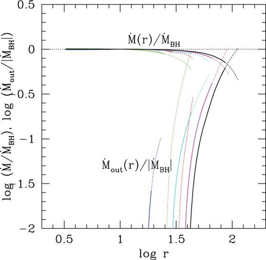
The horizontal lines near the top of the plot show the net mass inflow rate  for the six time chunks S1–S6 of the ADAF/SANE simulation, normalized by the net mass accretion rate on to the BH,
  . The colours and line types are as in Fig. 9. The vertical lines near the bottom show the variation of the mass outflow rate
  according to the μ criterion (the results are similar to those obtained with the Be or Be′ criteria), again normalized by
  . There is poor convergence in the results for the outflow, since no two successive time chunks are consistent with one another. The deviations are systematic – in the last three time chunks (S4: cyan, S5: magenta, S6: black), each successive time chunk gives a lower
  at a given r compared to the previous chunk. Hence, the mass outflow rates shown here should be interpreted as upper limits.
Fig. 9 indicates that there is a slow secular decrease in the converged values of both j and (1 − e) with time; the values for chunk S6 are smaller than those for S5, and so on. This is similar to, though not as extreme as, the declining trend in  already seen in Fig. 6. We suspect that, in the case of j and (1 − e), the reason for the decline is that the SANE simulation is slowly approaching the MAD limit (despite our best efforts to avoid it).
Fig. 10 shows equivalent results for the ADAF/MAD simulation. Here, j and (1 − e) are less well behaved than in the SANE simulation. In fact, it appears that even rstrict may overestimate the actual radius out to which inflow equilibrium has been achieved. The binding energy flux (1 − e) is a few times larger for the MAD simulation compared to the SANE simulation. This implies that the MAD accretion flow returns mechanical and magnetic energy to infinity more efficiently compared to the SANE simulation. In essence, the outflowing gas carries more energy per unit mass. The angular momentum flux j is substantially smaller in the MAD simulation compared to the SANE run. Indeed j appears secularly to approach zero with increasing time, as seen also in the highly sub-Keplerian values of uφ (compare Fig. 11 and 12). In fact, it seems that BH spinup via an ADAF/MAD accretion flow is highly inefficient. This agrees with the results reported in Tchekhovskoy et al. (2012) and McKinney et al. (2012).
Fig. 11 shows the radial velocity |vr(r)|, the specific angular momentum uφ(r) of the gas within one scale height and the normalized scale height h/r. There is good internal consistency between the profiles from successive time chunks. This is especially true when we focus only on the regions that satisfy the strict criterion for inflow equilibrium (the solid line segments). Specifically, apart from a tendency for h/r to increase slightly with time, the profiles of various quantities in successive time chunks line up well with one another, showing that we have a well-behaved accretion flow. We view the good agreement as a sign of convergence in our results.
At r = 100, we have |vr| ≈ 0.002, which is far smaller than the local free-fall velocity vff ≈ 0.14. This is to be expected. The radial velocity in a viscous flow is ∼α(h/r)2vff, where α is the dimensionless viscosity parameter and (h/r) is the dimensionless geometrical thickness of the disc. The simulated system has h/r ∼ 0.4 and α ∼ 0.05 (near r ∼ 100), and this explains the observed velocity.
The specific angular momentum uφ of the accreting gas is sub-Keplerian (as predicted by simple ADAF models). Interestingly, uφ continues to decline with decreasing radius even in the plunging region, i.e. inside the ISCO, rISCO = 6. It appears that the dynamics of an ADAF are not strongly modified when the gas crosses the ISCO. This is in contrast to geometrically thin discs, where the angular momentum becomes nearly constant once the gas flows inside the ISCO (Shafee et al. 2008; Penna et al. 2010).
The fourth panel in Fig. 11 shows the normalized Bernoulli-flux parameter μ (defined below in equation 13) of the mid-plane gas. Recall that the initial gas in the torus had Bernoulli in the range 10−2 to 10−3. The mid-plane gas in the accretion flow has a more negative value of μ, which means it is more tightly bound to the BH compared to the initial gas. The profiles from the different time chunks agree reasonably well with one another, but not perfectly. This is perhaps to be expected since μ is computed as the difference of two quantities of order unity. Note that the outflowing gas we consider in the next subsection has a positive μ. That gas has acquired extra energy in the process of accretion, and it is the extra energy that drives the outflow (Narayan & Yi 1994).
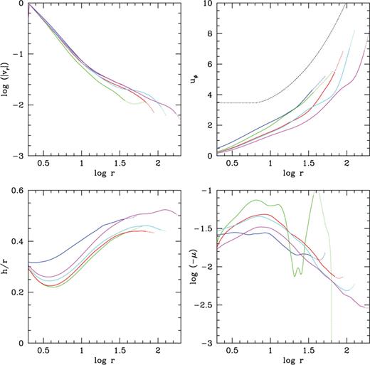
Fig. 12 shows the corresponding results for the MAD simulation. The radial velocity is substantially larger compared to the SANE simulation. Indeed, this is the reason for the larger zone of inflow equilibrium in this simulation. Both disc thickness h/r and Bernoulli Be show more fluctuations between successive time chunks. This is part of a pattern – fluctuations of all quantities are generally larger in the MAD simulation. The MAD flow is slightly thicker than the SANE flow, h/r ∼ 0.5 compared to ∼0.4, but it has roughly the same (negative) value of Be at the mid-plane.
3.2 Mass loss in an outflow
The main motivation behind the present study is to evaluate the amount of mass loss experienced by an ADAF through winds and outflows. Fig. 7 and 8 show that mass does flow out in both the SANE and MAD simulations. However, just because a given parcel of gas moves away from the BH does not necessarily mean that it escapes to infinity. The gas might just move out for a certain distance, turn round and merge with the inflowing gas. We need a physical criterion other than mere outward motion to determine whether or not mass is lost. Before proceeding further we note that there is no sign of a relativistic polar jet in our simulations, in agreement with the results of McKinney et al. (2012) for their runs with non-spinning BHs. This is perhaps not surprising since there is growing evidence that relativistic jets are powered by BH spin (Tchekhovskoy et al. 2011; Narayan & McClintock 2012). In any case, the discussion below is concerned with non-relativistic mass outflows, not jets.
We work with gas properties averaged over the duration of a time chunk tchunk and azimuthal angle φ, and symmetrized around the mid-plane. We do this not only for quantities like density and velocity, but also for all other quantities mentioned below, e.g. ρut, uut, b2ut, etc. As Fig. 7 and 8 show, such averaging eliminates all turbulent fluctuations inside the region of inflow equilibrium, allowing us to focus on the mean properties of the flow. This is important when trying to evaluate the magnitude of outflows.
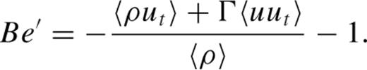
We have considered three criteria for deciding whether a gas streamline escapes to infinity. The first two criteria involve variants of the Bernoulli parameter of the gas. This was the parameter considered by Narayan & Yi (1994) in their original work in which they identified mass loss as being potentially important in ADAFs. In Newtonian hydrodynamics, Be is the sum of kinetic energy, potential energy and enthalpy. At large distance from the BH, the potential energy vanishes. Since the other two terms are positive, gas at infinity must have Be ≥ 0. Furthermore, in steady state and in the absence of viscosity, Be is conserved along streamlines. Hence any parcel of gas that flows out with a positive value of Be can potentially reach infinity. This was the crux of the argument proposed by Narayan & Yi (1994).
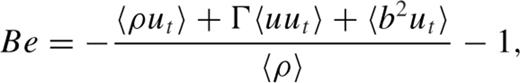
 is just a local version of
  in equation 2. Thus, μ measures the flux of the Bernoulli (normalized by mass flux) and is the most natural quantity for our analysis. In particular, it includes the contribution of the magnetic shear stress (terms like brbφ in equation 5), which is not included in the definitions of Be and Be′ above. As before, we consider a parcel of gas to escape to infinity from a given radius r if (1) its average velocity at r is pointed outwards, and (2) μ ≥ 0. For a steady axisymmetric ideal MHD flow, μ is conserved along an outflowing streamline. Hence this μ-based criterion is arguably the most physically well-motivated of the three criteria, and the one closest in spirit to the original work of Narayan & Yi (1994).
Using each of the three criteria described above, we have computed the mass outflow rate  as a function of r for each of the time chunks in the ADAF/SANE and ADAF/MAD simulations. The results from the three criteria agree well with one another. We show plots corresponding to only the μ criterion.
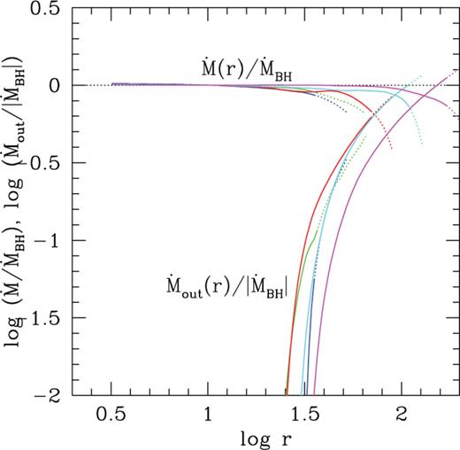
Fig. 13 shows for the ADAF/SANE simulation the mass outflow rate  and the net mass inflow rate
  , both normalized by the net mass accretion rate on to the BH,
  . The results for the mass inflow rate
  are identical to those shown in the top left panel of Fig. 6, except that the normalization by
  shifts the curves vertically and causes them to lie on top of one another.
Surprisingly, the results for  show very poor convergence. Specifically, the
  profiles corresponding to different time chunks deviate substantially from one another. Moreover, the deviations are systematic. In each time chunk, the outflow appears to pick up just around the limiting radius for inflow equilibrium. Since the latter moves out for later chunks, the entire
  profile also moves out. Apparently, at each time, the current estimate of the mass outflow rate at a given radius is an overestimate compared to the rate we would estimate at a later time (compare in particular the last three time chunks shown in cyan, magenta and black). Because of this, the outflow rate estimate even from the last time chunk S6 (black curve) must be viewed only as an upper limit. Moreover, even this estimate corresponds to a mass-loss rate at r ∼ 100 no more than the net inflow rate
  into the BH. Given that it is an upper limit, we can state with some confidence that mass outflow is unimportant for rH < r < 100.
It is useful to compare our results with those obtained by McKinney et al. (2012) for their model A0.0BtN10. This model was initialized with a toroidal field and is an excellent example of an ADAF/SANE system. In table 4 of their paper, the authors provide various estimates of the mass outflow rate measured at a characteristic radius ro = 50. Their quantity  is most relevant since it focuses on unbound gas, defined as Be′ > 0.7 The normalized mass outflow rate,
  , that McKinney et al. (2012) find at r = 50 in model A0.0BtN10 is essentially zero, in good agreement with our result,
  at r = 50 in chunk S6; at r = rstrict = 86, our outflow rate is
  . It should be noted that
  includes additional constraints, viz., that the escaping gas should have b2/ρ < 1 and gas to magnetic pressure ratio β < 2. Our mass outflow criteria do not include these constraints. When we include them, we find that our mass outflow rate is zero at r = 50 and 86. Apart from these details, both the present work and model A0.0BtN10 in McKinney et al. (2012) agree on the following key result: out to radii ∼50–100, ADAF/SANE systems have negligible mass outflow.
Fig. 14 shows mass outflow estimates obtained via the μ criterion for the ADAF/MAD simulation. As in the case of the ADAF/SANE simulation, the convergence behaviour is poor. In particular, the results from chunks M3 (red), M4 (cyan) and M5 (magenta) do not agree well with one another. Thus, once again, we believe the mass outflow rates we estimate from this simulation should be viewed as upper limits.
Mass outflow rate in the ADAF/MAD simulation based on the μ criterion. The colours and line types are as in Fig. 10. The last three chunks (M3: red, M4: cyan, M5: magenta) show large and systematic deviations, suggesting that (as in the case of the ADAF/SANE simulation) we do not have good convergence and the computed mass outflow estimates are upper limits.
Despite the unsatisfactory convergence, if we take the results at face value, we find for time chunk M5,  , 0.6, 1.1, at radii r = 50, 100, 170 (=rstrict), respectively. Two of the simulations described in McKinney et al. (2012), A0.0BfN10 and A0.0N100, correspond to MAD flows around non-spinning BHs and are good comparisons (though our simulation has run significantly longer). At radius ro = 50, A0.0BfN10 has essentially zero outflow, i.e.
  , while A0.0N100 has
  . Our estimate,
  , agrees well.8
We have looked a little deeper into why the  profiles we obtain from our simulations show poor convergence. Fig. 15 shows results corresponding to five streamlines in time chunk S6 of the ADAF/SANE simulation. These streamlines have footpoints at r = rstrict = 86 and θ = 0.2, 0.4, 0.6, 0.8, 1.0 rad, respectively. All these streamlines have a positive value of μ at their footpoints. Since μ is supposed to be conserved along each streamline, all of this gas ought to escape. The right-hand panel of Fig. 15 shows the variation of μ along each streamline as the gas moves away from the BH. We see that μ is approximately constant and positive for the three streamlines closest to the pole. However, the two streamlines closer to the disc show a sudden drop in the value of μ as one moves outwards. Clearly these streamlines have not reached steady state, since μ would then be constant. It seems likely that the positive value of μ for these streamlines is a transient feature. Unfortunately, these suspect streamlines carry the most mass.
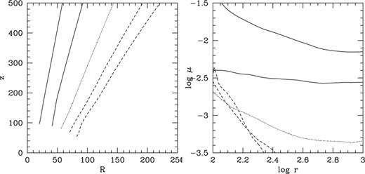
Left: five outflowing streamlines in time chunk S6 of the ADAF/SANE simulation. The streamlines have their footpoints at (r, θ) = (86, 0.2), (86, 0.4), (86, 0.6), (86, 0.8), (86, 1.0). All five streamlines have positive values of μ at their footpoints. Right: the variation of μ along each of the streamlines in the left panel, using the same line types. Note that μ shows large deviations from constancy for the last two streamlines.
Fig. 16 shows similar results for four outflowing streamlines in the ADAF/MAD simulation. Here the conservation of μ along outgoing streamlines is satisfied much better. In addition, the value of μ is generally larger, which indicates that the outflowing gas carries more energy per unit rest mass.
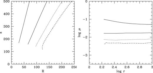
Similar to Fig. 15, but for the ADAF/MAD simulation. The streamline footpoints are at (r, θ) = (170, 0.2), (170, 0.4), (170, 0.6), (170, 0.8). All four streamlines have positive μ at their footpoints, and all show good conservation of μ.
3.3 Convection
A secondary goal of this study is to investigate the importance of convection in magnetized ADAFs. It is well-known that the entropy profile in an ADAF has a large negative gradient, making the flow highly unstable by the Schwarzschild criterion. However, an ADAF also has angular momentum increasing outwards, which has a stabilizing effect on convection.
For axisymmetric rotating flows, the two Hoiland criteria determine whether or not gas is convectively unstable. The same criteria are likely to remain approximately valid also in magnetized flows, so long as the field is reasonably weak, since the long-wavelength convective modes are effectively hydrodynamical (Narayan et al. 2002). In addition, since convection is a local instability, the relativistic versions of the Hoiland criteria (Seguin 1975) carry over directly to general relativity by the equivalence principle.
We have analysed the final time chunk S6 in the ADAF/SANE simulation to determine the level of convective instability in the accretion flow. Fig. 17 shows the result. In brief, all the fluid within two scale heights of the mid-plane appears to be convectively stable. The gas is certainly turbulent (see Fig. 4) – this is what enables it to accrete – but it is apparently not convective, at least by the Hoiland criteria. Rather, the turbulence seems to be entirely the result of the MRI. Could magnetic fields be confusing the issue? We think this is unlikely. Analytical studies of convection in the presence of magnetic fields (Balbus & Hawley 2002; Narayan et al. 2002) show that magnetic fields generally act in such a way as to stabilize convection. That is, a fluid configuration that is convectively unstable could be made stable by a suitable field, but not the other way round. Of course, the magnetic field might induce its own instability, e.g. MRI, but this can no longer be considered convection. We intend to explore this question in greater depth in the future.
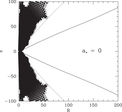
Analysis of convective stability of the ADAF/SANE simulation. Results are shown for time chunk S6 using time- and azimuth-averaged, symmetrized, simulation data. At each point (R, z) in the poloidal plane, the maximum growth rate γ according to the two Hoiland criteria is computed. Stable regions are shown by blank areas. Unstable regions where γ < ΩK/30 are indicated by crosses, regions with ΩK/30 ≤ γ < ΩK/10 are indicated by open circles, and regions with γ ≥ ΩK/10 are indicated by filled circles. The solid and dotted lines correspond to one and two density scale heights, respectively. Note that the accretion flow is stable to convection over the entire inflow region. The instability near the poles is not significant since the analysis is not valid there.
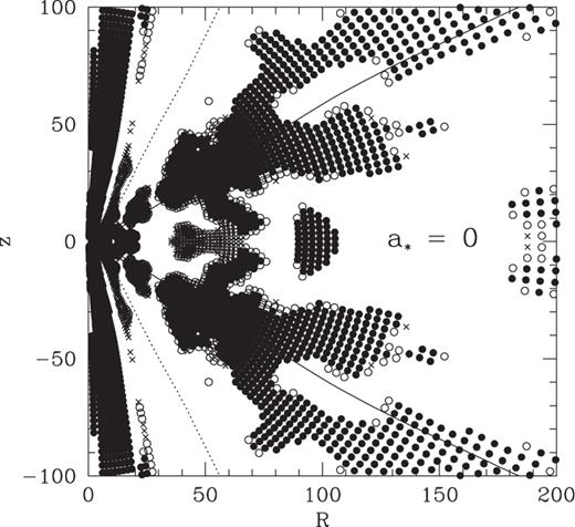
Fig. 18 shows the convection properties of the ADAF/MAD simulation. Based on the Hoiland criteria, it appears that the MAD simulation is more unstable to convection compared to the ADAF/SANE simulation. This is not surprising. The gas rotates much more slowly and hence the stabilizing effect of rotation, which we think is the primary reason for the lack of convection in the ADAF/SANE simulation, is no longer effective. We caution, however, that the magnetic stress is larger in the MAD simulation, and the Hoiland criteria do not include the effect of this stress. By the argument in the previous paragraph, the magnetic field might well be strong enough to switch off the convective instability even in those regions where the Hoiland criteria indicate instability. The accreting gas in the MAD simulation has very little turbulence, so it certainly does not manifest any of the usual features of turbulent convection. We suspect that the flow is in a state of frustrated convection as proposed by Pen et al. (2003).
4 Adaf or CDAF or Adios?

 is the steady mass accretion rate, α is the viscosity parameter, Ω is the angular velocity and Γ is the adiabatic index. These scalings follow from basic conservation laws and the α prescription for viscosity. By assumption, there is no mass outflow.

 . Recently, Begelman (2012) has presented arguments suggesting that s ≈ 1.
All of the above models are based on a fluid description, without allowing explicitly for magnetic fields. We believe this is reasonable, at least for the ADAF/SANE simulation, where the magnetic stress behaves to a good approximation like viscosity, and the magnetic pressure is not very important relative to gas pressure. Akizuki & Fukue (2006) have developed self-similar solutions for magnetized ADAFs. However, they assume a purely toroidal field (no shear stress) and consequently have to invoke α-viscosity. Moreover, their solutions are similar to the ADAF/ADIOS solutions mentioned above so long as the magnetic pressure is modest, as in the ADAF/SANE simulation. This last condition may not be true for the ADAF/MAD simulation. However, even for a MAD flow, the model of Akizuki & Fukue (2006) is not appropriate since it assumes a toroidal field, whereas the key feature of the MAD solution is a strong poloidal field.
We have shown in Section 3 that the ADAF/SANE and ADAF/MAD simulations appear not to be convective, to the extent we can tell from the Hoiland criteria. We did not include the effect of the magnetic field, so we cannot make any firm statements regarding convection. Nevertheless, for the present, we will assume that neither simulation is a full-fledged CDAF. Also, neither flow has significant mass outflow up to r ∼ 100. We can thus say that the simulations are best described as ‘basic’ ADAFs9 over this radius range, though it is possible that they are just beginning to make a transition to the ADIOS state beyond r = 100. From equations 14 and 16, we see that both solutions predict |vr| ∼ αr−1/2, which can be checked.
The left-hand panel in Fig. 19 shows the velocity profiles in the final time chunks, S6 and M5, of the ADAF/SANE and ADAF/MAD simulations. There is some indication that, at the outermost radii of the respective converged regions, the velocity is settling to the expected r−1/2 dependence. However, over most of the flow, the velocity varies more steeply with radius. Part of the explanation is that, in the self-similar regime, the radial velocity of an ADAF is approximately given by |vr| ∼ α(h/r)2vff ∼ 10−2vff. However, at the BH horizon the gas must have |vr| = vff = c. The radial velocity thus has to transition from its self-similar value to the free-fall value. It takes a substantial range of r to achieve this, especially in the ADAF/SANE simulation. The radial velocity in the MAD simulation is larger, |vr| ∼ 0.1vff, so this flow is able to follow the self-similar scaling closer to the BH.
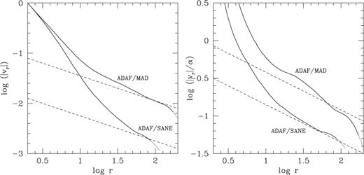
Left: radial velocity |vr(r)| of the gas in time chunk S6 of the ADAF/SANE simulation (from Fig. 11) and time chunk M5 of the ADAF/MAD simulation (from Fig. 12). The two dashed lines have slope equal to −1/2, the value expected in the self-similar regime for both a basic ADAF and an ADIOS. Over most of the volume, the velocity varies more rapidly with radius than expected for a self-similar solution. Right: similar to the previous panel, but showing the quantity |vr(r)|/α(r). Note that the ADAF/SANE model agrees much better with the self-similar model, except as the gas approaches the ISCO (rISCO = 6).
A second effect is also in operation, viz., the effective α of the accreting gas varies with r. The right-hand panel in Fig. 19 corrects for this by plotting |vr|/α, where α(r) is estimated directly from simulation data for gas within one density scale height of the mid-plane. The ADAF/SANE simulation now shows satisfactory self-similar behaviour over a wider range of r. Removing the α scaling does not improve things much for the ADAF/MAD simulation.
All of this discussion is based on the radial velocity vr(r), which we feel is the natural dynamical variable to consider. Most previous authors have focused instead on the density profile ρ(r). In steady state the two quantities are simply related: 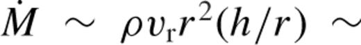 constant. The mid-plane density profiles in our two simulations are roughly compatible with the velocity results shown in Fig. 19. Many authors, notably Yuan et al. (2012b), find that the density follows a single power law over a wide range of radius. The velocity does not show this property (Fig. 19).
Fig. 20 shows the dependence of the gas angular velocity Ω in our two simulations. The ADAF/SANE simulation shows excellent convergence in the sense that the Ω(r) curves from different time chunks agree very well with one another. Moreover, the angular velocity follows the analytical r−3/2 scaling quite accurately. However, the normalization is not correct. Since Γ = 5/3, the self-similar ADAF model predicts Ω ∼ 0 (see equation 14), whereas we find distinctly non-zero rotation in our simulation.
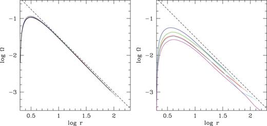
Left: angular velocity Ω(r) of the gas in time chunks S1–S6 of the ADAF/SANE simulation. The dashed line has a slope equal to the self-similar value of −3/2. Right: similar plot corresponding to the five time chunks M1–M5 of the ADAF/MAD simulation.
The likely explanation is that the simulation behaves, not like the steady-state self-similar solution of Narayan & Yi (1994), but rather like the similarity solution derived by Ogilvie (1999). The latter solution describes the evolution of an advection-dominated flow as a function of both r and t, starting from an initial narrow ring of material. With increasing time, the flow evolves in a self-similar fashion. Most interestingly, in Ogilvie's solution, the angular velocity does not go to zero anywhere except in the region r → 0. In fact, over most of the volume, the rotation rate remains a substantial fraction of the Keplerian rate, exactly as in our simulations. Since we started our simulations with an initial torus of material, the similarity solution is a better point of reference than the self-similar solution; the latter is valid only at asymptotically late time when the flow has reached steady state at all r.
As a further comparison between the ADAF/SANE simulation and Ogilvie's (1999) similarity solution, Fig. 21 displays again the radial velocity profiles for different time chunks, but now shown over an extended range of radius. The velocity in each profile dives suddenly to zero and becomes negative at a ‘stagnation’ radius rstag. We see that rstag increases with increasing time, as expected for the similarity solution. The analytical solution predicts rstag ∝ t2/3, which means that rstag should increase by a factor of ∼10 between chunks S1 and S6. The actual increase is a factor of 20. We view this as good agreement.
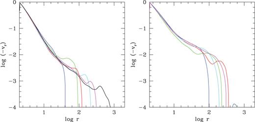
Left: radial velocity versus r for time chunks S1–S6 of the ADAF/SANE simulation. The colour code is the same as in Fig. 9. Note that each curve dives down suddenly at a certain radius. This is the stagnation radius for that time chunk. Beyond this radius, the mean velocity is outwards because of the viscous relaxation of the initial torus. Right: corresponding results for the ADAF/MAD simulation, with colour code as in Fig. 10.
The ADAF/MAD simulation results shown in the right-hand panels of Fig. 20 and 21 are less convincing. This simulation has a strong magnetic field and an arrested mode of accretion which, based on the evidence of all the diagnostics plotted in various figures, makes the flow behave more erratically. Analytically, the MAD regime is sufficiently different from the SANE regime that we cannot expect either the self-similar ADAF solution or Ogilvie's similarity solution to be a good description.
As already stated, there is a hint near the outer edges of the ADAF/SANE and ADAF/MAD simulations that ADIOS-like behaviour is beginning to take hold. If we had a larger range of radius in inflow equilibrium, it might be possible to estimate how the outflow rate varies with radius and thereby determine the index s in the scaling  . Unfortunately, this is out of reach with our current simulations. Yuan et al. (2012b) estimate from their large dynamic range 2D hydrodynamic simulations that s ∼0.4–0.5.
5 Summary and Discussion
The main highlights of the present work are: (1) we have run our simulations for an unusually long time in an effort to approach a steady-state ADAF as closely as possible over a wide range of radius. (2) We have explored the role of the initial magnetic field topology. With respect to the latter, we have considered two very different limits: (1) an ADAF/SANE simulation (SANE = ‘standard and normal evolution’), which is a good proxy for an ADAF model in which the magnetic field is merely an agent that causes angular momentum transport (‘viscosity’) but plays no important dynamical role, and (2) an ADAF/MAD simulation (MAD = ‘magnetically arrested disc’), where the magnetic field is strong enough to alter substantially the dynamics of the gas and to drive the system to a magnetically arrested state (Igumenshchev et al. 2003; Narayan et al. 2003; Tchekhovskoy et al. 2011; McKinney et al. 2012).
Our key result is that, for radii out to r ≈ 100 (gravitational units, GM/c2), there is not much mass loss to an outflow. Turbulence certainly leads to both inward and outward gas motions. However, when we consider the time-averaged gas flow and how much gas flows out with enough energy to escape from the gravitational potential of the BH, it turns out to be only a fraction of the net mass accretion rate  into the BH. Quantitatively, at r ≈ 100, we find
  for both simulations. Furthermore, we view these estimates as upper limits since the simulations reveal poor convergence in
  (see Fig. 13 and 14).
Because of the very long run times of our simulations, we are unable to run multiple realizations of the SANE and MAD configurations to explore variability from one realization to another. On the other hand, the long run time allows us to explore convergence as a function of time within each simulation. We do this by dividing the simulation data into a number of independent chunks in log t (Section 2.3 and Tables 1 and 2). By comparing different time chunks and checking how any quantity of interest varies from one chunk to the next, we are able to decide how reliable the results are for that quantity.
A second important issue is the range of r over which each time chunk has reached inflow equilibrium. We use two different criteria, a strict one (equation 9) and a loose one (equation 10), and estimate for a given chunk the limiting radii, rstrict and rloose, corresponding to each of these criteria (Tables 1 and 2). Many properties of the gas show good convergence among different time chunks when we limit our attention to radii r ≤ rstrict. The results are less convincing with the loose criterion. However, even with the strict criterion, we find that some questions such as the amount of mass loss in outflows cannot be answered with confidence.
We initialized the ADAF/SANE simulation with a number of poloidal magnetic loops (Fig. 2) in an attempt to achieve an accretion flow with very little net flux at each radius. By and large this simulation behaved the way we hoped it would. In particular, the magnetic flux at the BH horizon, measured by the parameter φBH, did not come close to the limiting MAD value of 50 (except for one brief glitch at time t ∼ 140 000; see Fig. 5). Thus we believe the ADAF/SANE simulation is a believable representation of an ADAF system. We could have avoided the MAD regime more effectively by starting the simulation with a purely toroidal field, as in Model A of Igumenshchev et al. (2003) or Model A0.0BtN10 of McKinney et al. (2012). This option is worth exploring in the future.
The ADAF/SANE simulation shows good convergence and behaves as expected. The radial velocity, angular velocity, angular momentum and disc thickness profiles as a function of r agree well between different time chunks (Fig. 11 and 20). At large radii, the radial velocity falls well below free-fall (Fig. 19). This is expected since accretion is mediated by ‘viscous’ angular momentum transport which causes the velocity to be suppressed by a factor of α relative to free-fall; there is also a factor of (h/r)2 which causes a further decrease in the velocity. Interestingly, as discussed in Section 4, the ADAF/SANE simulation is better described by the similarity solution of Ogilvie (1999) than the original self-similar solution of Narayan & Yi (1994). Nevertheless, the radial dependence of velocity follows the self-similar solution quite well (Fig. 19, right-hand panel).
The ADAF/MAD simulation shows quite different behaviour compared to the ADAF/SANE simulation. The inflow velocity is substantially larger and the angular momentum and angular velocity are substantially smaller (Fig. 12 and 20). The latter appears to be an important characteristic of MAD flows. As discussed in Tchekhovskoy et al. (2012), the gas brings in very little angular momentum to the BH and therefore induces little spin-up even for a non-spinning BH. In the case of a spinning BH, a MAD flow actually causes spin-down. The reduced rotation rate of the gas means that there is less centrifugal support. Consequently, the radial dynamics are dominated by balance between gravity, gas pressure and magnetic stress. We find that the gas accretes at about a tenth of the free-fall speed, which is a factor of several larger than the velocity in the ADAF/SANE simulation.
Because of the larger radial velocity, the ADAF/MAD simulation reaches inflow equilibrium over a substantially larger range of radius at a given time relative to the ADAF/SANE simulation (compare Tables 1 and 2). On the other hand, convergence in the sense of agreement between different time chunks is less convincing. We suspect that the reason is the large-scale ordered magnetic field in the MAD simulation, which imposes coherent long-lived structure in the flow.
In terms of the amount of mass outflow, the ADAF/SANE and ADAF/MAD simulations behave rather similarly. We tried three different criteria to determine how much gas escapes to infinity at a given radius: one criterion was based on the Bernoulli parameter Be (equation 11), a second on a different Bernoulli Be′ that ignores the magnetic contribution (equation 12) and a third on the normalized energy flux μ (equation 13). The results are nearly identical with all three criteria, which is reassuring. Unfortunately, the results show poor convergence with time. In particular, the radial variation of  for the last few time chunks (S4–S6 and M3–M5) differs by much more than we would expect for a converged simulation. Nevertheless, taking the results at face value, we conclude that the mass outflow rate
  becomes comparable to the net inflow rate
  into the BH at a radius r ∼ 120 = 60rH in the ADAF/SANE simulation and r ∼ 160 = 80rH in the ADAF/MAD simulation. These radii are fairly far from the BH. In fact, since our mass outflow rates are upper limits, the critical radii where mass outflows begin to dominate could be substantially larger.
Our result that outflows are weak out to r ≳ 100 disagrees strongly with previous work. Many simulations of ADAFs have been described in the literature (see Section 1 for a brief review), and most of these studies have concluded that there are powerful mass outflows at radii well below r = 100. On investigation, it appears that there is a significant methodological difference between our approach and that used by previous authors. As explained in Section 3.2, all of our calculations are based on time- and azimuth-averaged quantities in which fluctuations due to turbulence have been eliminated. Only if the average velocity of gas in a grid cell has a positive radial component, and furthermore if the gas has enough energy to escape from the system (μ > 0), do we consider the particular gas packet to be part of an outflow. Most other authors have focused on individual snapshots of their simulations and counted any gas that happened to be moving away from the BH as outflow. Since turbulence causes gas to move to and fro, a good fraction of the gas in any snapshot would be moving out simply as part of turbulent eddies. However, very little of this gas would actually leave the system since the velocity vector is likely to turn round on an eddy time. Moreover, much of the gas would probably have insufficient energy (μ < 0) to climb out of the BH potential. Indeed, several previous authors have noted, after presenting very large estimates for the mass outflow rate, that most of the gas in their ‘outflows’ has a negative Bernoulli.
The distinction between the approach taken in previous papers and in the present work can be appreciated by comparing Fig. 4 and 7. The snapshot of the ADAF/SANE simulation in the left-hand panel of Fig. 4 shows turbulent eddies down to quite small radii. A fraction of the gas in each of these eddies is temporarily moving outwards, but none of it is likely to escape to infinity. However, in the standard approach used to estimate the mass outflow rate, the outward-moving part of each eddy would be included as part of  . This is likely to lead to a large overestimate of the mass outflow rate. In contrast, our calculations use the average flow streamlines shown in Fig. 7. Consider the final time chunk S6 (lower right panel). Inside r ∼ 30–40, there are no streamlines with velocity vectors pointed away from the BH. Therefore, when we compute the mass outflow rate, we obtain vanishingly small values of
  for radii ≲30 (Fig. 13).
Because of the above major difference between our calculations and those of previous authors, it is hard to compare our results. The one exception is McKinney et al. (2012), who, though basing their work on snapshot data, explain their calculations in sufficient detail to enable a comparison. Leaving aside jets, which are not relevant for the non-spinning BHs considered here, McKinney et al. (2012) present two distinct estimates of the mass outflow rate. One estimate is called  , and it focuses on outflowing gas with positive Be′ (it also imposes a couple of other constraints; see Section 3.2). This quantity is closest to our prescription for estimating the mass outflow. Their second outflow estimate is called
  , and it includes essentially all outflowing gas in each snapshot, independent of Be. This quantity is close in spirit to mass outflow estimates in many other papers in the literature, and is in our view an overestimate of the actual mass-loss rate because it includes gas churning in turbulent eddies.
For their Model A0.0BtN10, which is an excellent example of an ADAF/SANE system around a non-spinning BH, McKinney et al. (2012) estimate  at r = 50 (here
  is the net mass accretion rate into the BH, similar to our
  ), which suggests a strong outflow already at this radius. However, they find
  to be essentially zero. In our ADAF/SANE simulation, at r = 50 we find
  , i.e. practically zero, in good agreement with
  . In the case of their two ADAF/MAD systems around non-spinning BHs, A0.0BfN10 and A0.0N100, McKinney et al. (2012) find at r = 50 that
  , 0.4, and
  , 1.1, respectively. Our ADAF/MAD simulation gives
  , in agreement with the
  estimates. It thus appears that our results are perfectly compatible with the work of McKinney et al. (2012). We are also in agreement with Pang et al. (2011), though the latter work is mostly concerned with the accretion of slowly rotating gas.
Some papers have argued for strong outflows based simply on the fact that the radial profile of density and/or velocity do not follow the standard ADAF scalings given in equation 14. Focusing on the radial velocity, the simulations generally show |vr| increasing more rapidly with decreasing radius than expected in the self-similar solution. Our simulations too show this effect (Fig. 19). It turns out that two separate effects, neither involving outflows, cause the velocity profile to be modified.
First, because the accreting gas makes a sonic transition as it approaches the BH and switches to a free-fall mode inside this radius, we have |vr| ∼ vff near the BH. However, the velocity in the self-similar regime is far below free-fall: |vr| ∼ α(h/r)2vff. The flow needs a considerable range of r to adjust from one scaling to the other, and we believe this is a large part of the reason why the velocity profiles seen in simulations look so different from the simple power law given in equation 14. Clear examples of this effect may be seen in the global 1D models of Narayan, Kato & Honma (1997), where the non-self-similar zone extends from the inner boundary to a few tens of gravitational radii.
Secondly, it is the quantity vr/α that is expected to be self-similar, not vr itself. Since α varies with radius in our simulations (especially in the ADAF/SANE simulation), this causes an additional deviation in vr(r). As Fig. 19 shows, removing the α dependence gives a better behaved velocity profile that agrees fairly well with the models shown in Narayan et al. (1997).
Another argument for strong outflows that is sometimes used in the literature is to take the gas density at the outer radius of the simulation, and to calculate from it the Bondi mass accretion rate  . If the actual mass accretion rate
  into the BH in the simulation is much smaller than
  , then it is claimed that the difference is because most of the incoming gas was ejected in an outflow. The problem with this argument is that, for a given outer boundary condition on the density, theory says that the accretion rate via an ADAF will be smaller than
  by a factor ∼α(h/r)2 ∼ a few per cent. Thus, having
  is perfectly natural for an ADAF; it does not imply strong outflows. Note, however, that this explanation only goes so far. If it turns out that
  is much smaller than even
  , then one has to look for other explanations such as strong outflows or convection. To our knowledge, no simulation to date has come close to violating this limit.
ADAFs in nature usually extend over many decades in radius. The ADAF around Sgr A*, for instance, extends from the BH out to the Bondi radius at r ≳ 105. Supermassive BHs in other low-luminosity active galactic nuclei similarly have ADAFs extending over five or more decades in radius. In the case of stellar-mass BHs in X-ray binaries, the ADAF is usually formed by evaporation from a thin disc on the outside (Narayan & McClintock 2008). For systems in quiescence, where the mass accretion rate is low, the transition radius is typically ∼103−104. In contrast, simulations of ADAFs are generally restricted to a much smaller range of radius (but see the recent work of Yuan et al. 2012b). How relevant are simulation results to real systems?
Our views on this question are driven by insights gained from global 1D models of ADAFs such as the ones shown in Narayan et al. (1997) and Chen, Abramowicz & Lasota (1997). These solutions show three zones: an inner zone where the flow adjusts to the free-fall boundary condition at the BH, an outer zone where it adjusts to whatever outer boundary condition is present in the system (Bondi or disc evaporation) and a middle zone where the flow is more or less self-similar. If a simulation covers a large enough radius range to capture some piece of the middle zone, then it would be straightforward to stretch out the self-similar regime to any radius range we require. We suspect that the two simulations presented in this paper may have just managed to develop a piece of the middle zone, but we do not have any proof of this. In any case, we believe that only by obtaining inflow equilibrium over a sufficiently large range of radius can we hope to use simulations to make useful statements about real flows.
It should be noted that the properties of the self-similar middle zone are fairly insensitive to parameters. There is an obvious dependence on α (see equation 14) and a modest dependence on Γ,10 but virtually nothing else matters. In other words, provided ADAF conditions are satisfied, the accretion flow will head towards the particular disc thickness h/r and Bernoulli Be(r) it wants in the middle zone, regardless of the precise outer boundary conditions. This is demonstrated for instance in fig. 5 of Narayan et al. (1997), where three very different outer boundary conditions on the gas rotation and temperature all give pretty much identical solutions in the middle zone. The same is true also for Be (fig. 7 of the same paper). Yuan et al. (2012a) have carried out hydrodynamic simulations of ADAFs where they find that Be of the accreting gas is mainly set by the outer boundary condition. It is possible that their models do not extend over a large enough range of radius to sample the self-similar zone.
All the results presented here refer to a non-spinning BH. This is the simplest version of the ADAF problem, where there is no additional complication from central energy injection by a spinning BH. It is also the case that relates most directly to theoretical work as well as to non-relativistic MHD simulations. In the case of ADAFs around spinning BHs, although a large fraction of the energy from the BH seems to go out in a relativistic jet (Tchekhovskoy et al. 2011), some of it presumably propagates into the accreting flow. This energy very likely will induce extra mass loss, as seen in the simulations described by Tchekhovskoy et al. (2011) and McKinney et al. (2012). Sorting out the BH spin effect from the intrinsic effect due to ADAF physics is left for future work.
In addition to outflows, we have also described in this paper a preliminary analysis of convection. In brief, the ADAF/SANE simulation shows no evidence of convective instability (Fig. 17), while the ADAF/MAD simulation is apparently unstable by the Hoiland criteria over a part of its steady-state region (Fig. 18). However, there is little evidence in the MAD simulation for actual turbulent convection. Hence we speculate that the ADAF/MAD simulation is probably in a state of frustrated convection (Pen et al. 2003). Based on our current results, we are inclined to think that convection is unimportant in ADAFs, whether SANE or MAD, but this issue needs to be investigated in greater detail before one can be certain. In particular, it is important to sort out the effect of the magnetic stress, which is ignored in the Hoiland criteria. Also, it is possible that the accretion flow is described by something like the global 1D models in Abramowicz et al. (2002), where the flow behaves like a basic ADAF (no outflow, no convection) until a radius r ∼ 35 rH = 70, and then switches to a CDAF. We do not have enough dynamic range in our ADAF/SANE simulation to rule this out.
We note that there are some observational indications against strong mass loss in ADAFs. Allen et al. (2006) showed that a number of low-luminosity active galactic nuclei have radio jets with implied powers that are a reasonable fraction of accretion energy at the Bondi rate from the surrounding interstellar medium. In fact, McNamara et al. (2011) identified systems with  , and argued that these jets must be powered by BH spin. While it is true that a rapidly spinning BH can produce a very strong jet, the jet power is still linked to the accretion power; Pjet may be a factor of a few larger than
  , but not much more (Tchekhovskoy et al. 2011; McKinney et al. 2012). Therefore, the observations mentioned above mean that a good fraction of the available mass at the Bondi radius must reach the BH (Narayan & Fabian 2011). If mass loss between the Bondi radius and the BH is very large, as in some versions of the ADIOS model (Blandford & Begelman 1999; Begelman 2012), or if a CDAF is present over a wide range of radius, there would not be sufficient mass near the BH to tap the BH spin energy and power the observed jets. We believe that the above observational evidence, assuming it holds up, drives us towards one of the following descriptions of the accretion flow: (i) an ADAF with a weak outflow, i.e. a value of the index s close to 0, or (ii) an ADAF with a strong outflow (s ≈ 1) but with the outflow restricted to a small range of radius, say no more than one or two decades, or (iii) a CDAF with properties and scalings rather different from the analytical models in the literature (Narayan et al. 2000; Quataert & Gruzinov 2000b), or (iv) a perfectly spherically symmetric Bondi flow. We consider the fourth possibility unlikely since it requires gas at the Bondi radius to have an extremely low specific angular momentum.
The interesting differences we find between the ADAF/SANE and ADAF/MAD simulations brings up the question of which is more relevant for real systems. The defining feature of a MAD system is that accretion has dragged in a considerable amount of magnetic flux and has caused the field to accumulate around the BH. Whether or not accretion can drag field so effectively has been much debated (e.g. Lovelace, Rothstein & Bisnovatyi-Kogan 2009; Guilet & Ogilvie 2012, and references therein), but it is agreed that field-dragging will be most efficient in thick accretion flows such as ADAFs rather than in thin discs. Assuming that inward advection of magnetic field does operate effectively in ADAFs, there is typically more than enough magnetic field available in the external medium to drive an accreting BH to the MAD state (Narayan et al. 2003).
Acknowledgments
The authors thank Jonathan McKinney, Re'em Sari, Alexander Tchekhovskoy and Feng Yuan for comments on the paper. This work was supported in part by NASA grant NNX11AE16G and NSF grant AST-0805832. The simulations presented in this work were performed on the Pleiades supercomputer, using resources provided by the NASA High-End Computing (HEC) Program through the NASA Advanced Supercomputing (NAS) Division at Ames Research Center. We also acknowledge NSF support via XSEDE resources at NICS Kraken and LoneStar.
References
Actually, two distinct ADAF modes are possible, one in which optically thin two-temperature gas accretes with a highly sub-Eddington Ṁ, and a second in which very optically thick radiation-trapped gas accretes at rates well above the Eddington rate. We are concerned in this paper with the former kind of ADAF, which our GRMHD code is capable of simulating. The latter variety of ADAF is referred to as a ‘slim disc’ (Abramowicz et al. 1988) and requires a radiation MHD code to simulate (see Ohsuga et al. 2009; Ohsuga & Mineshige 2011; and references therein).
As it happens there is no significant jet in the simulations described here. However, we plan to use the same grid setup and initial conditions in future work with spinning BHs, where we do expect to see strong jets.
In the notation of Penna et al. (2012), the ADAF/SANE magnetic field has rstart = 25M, rend = 550M and λB = 2.5. The ADAF/MAD magnetic field has rstart = 25M, rend = 810M and λB = 25.
The reason for choosing r = 10 rather than r = rH is to avoid small deviations that sometimes arise near the horizon because of the activation of floors in the harm code. Since r = 10 is well inside the inflow equilibrium zone at all times of interest, it is a safe choice.
Obviously, more accurate results could be obtained by using an even stricter criterion, e.g. tvisc ≤ tchunk/4. However, this would reduce the range of r so much that we would not have sufficient dynamic range to obtain any useful results.
The authors define a second quantity, Ṁw, o, which represents all outflowing gas, regardless of whether the Bernoulli is positive or negative. It is less relevant for us since most of this gas is bound to the BH and cannot escape to infinity. We thank J. McKinney (private communication) for clarifying the definitions of Ṁmw, oṀw, o.
As mentioned earlier, McKinney et al. (2012) require several conditions to be satisfied, viz., vr > 0, Be′ > 0, b2/ρ < 1, β < 2, before they include a particular gas streamline in their estimate of  . When we apply the same conditions on our ADAF/MAD simulation, we estimate the mass outflow rate at r = 50 to be 0.06, still in good agreement with their outflow rates.
By ‘basic ADAF’ we simply mean an ADAF that has no convection and no significant outflows. Systems with convection (CDAFs) and strong outflows (ADIOS) are still ADAFs in the general sense of the term, but they are not ‘basic ADAFs’.
In the low- RIAF branch of ADAFs, it is believed that the gas is two-temperature with non-relativistic ions and relativistic electrons (Narayan & McClintock 2008). If we take Te/Ti = 0.1, a reasonable value for an ion-dominated ADAF, then we expect Γ = 1.61. In the simulations presented here we have set Γ = 5/3, which is close enough, although technically in the ‘unphysical region’ discussed by Mignone & McKinney (2007). In the ADAF literature, Γ = 1.5 is often used, but this is because those models wish to include the effect of a tangled magnetic field, which has an effective Γ = 4/3. In numerical MHD simulations, the magnetic field is treated as an independent component, so we are only concerned with the gas. Any choice Γ ≳ 1.6 is probably reasonable.
