Astrometric and photometric initial mass functions from the UKIDSS Galactic Clusters Survey – II. The Alpha Persei open cluster

Abstract

1 INTRODUCTION

The shape of the initial mass function (IMF) is of prime importance to understand the processes responsible for the formation of stars and brown dwarfs. The definition and the first estimate of the IMF was presented in Salpeter (). Our knowledge of the IMF has now improved both at the high-mass and low-mass ends. The mass spectrum in open clusters and in the field, defined as dN/dM ∝ M^−α (α is the exponent of the power law and equivalent to x + 1, where x is the slope of the logarithmic mass function), is currently best fitted by a three-segment power law with α = 2.7 for stars more massive than 1 M_⊙, α = 2.2 between 1 and 0.5 M_⊙ and α = 1.3 ± 0.5 in the 0.5–0.08 M_⊙ mass range (Kroupa ). Alternatively, a log-normal function with a characteristic mass around 0.2–0.25 M_⊙ and dispersion ∼0.55 (Chabrier , ) provides a good match to current observations for the system mass function in the field. The advent of large-scale optical and near-infrared surveys towards open clusters extended the mass spectrum to the substellar regime but a consensus has yet to emerge on the detailed shape.

α Per is one of the few open star clusters within 200 pc of the Sun and younger than 200 Myr. The cluster is located to the north-east of the F5V supergiant Alpha Persei at a distance of ∼175–190 pc (Pinsonneault et al. ; Robichon et al. ) with a revised distance of 172.4 ± 2.7 pc from the re-reduction of the Hipparcos data (van Leeuwen ). The cluster members have solar metallicity (Boesgaard & Friel ) and the extinction along the line of sight is estimated as A_V = 0.30 mag with a possible differential extinction (Prosser ). It has been well studied, though less frequently than the Pleiades due to a smaller proper motion ((μ_αcos δ, μ_δ) = (+22.73,−26.51) mas yr⁻¹; van Leeuwen ) and a much lower galactic latitude (b = −7° versus −24°). Despite being further away than the Pleiades (170 pc versus 120 pc), α Per is a good target for substellar studies because it is younger than the Pleiades (85 ± 10 Myr versus 125 ± 8 Myr), placing the lithium depletion boundary at I_c ∼ 17.7–17.8 mag for both clusters.

Multi-wavelength surveys and spectroscopic follow-up observations have been performed in α Per to extract a clean sequence of cluster members from high-mass stars down to brown dwarfs. The first proper motion survey in the cluster was performed by Heckmann, Dieckvoss & Kox () and complemented by photometry from Mitchell (), yielding about 60 probable members (HE objects) whose final membership was revised by Prosser (). The membership of additional candidates proposed by Fresneau () was subsequently established by Prosser (). Lower mass members (AP sources) were extracted by Stauffer et al. () and Stauffer, Hartmann & Jones () on the basis of their proper motion, photometry and spectral characteristics. Prosser () examined the Palomar photographic plates to extract new low-mass proper motion and photometric members down to a spectral type of M4 over a 6° by 6° field. Additional low-mass photometric candidates were reported from a deeper optical survey in a smaller area (Prosser ) as well as from X-rays observations with ROSAT (Prosser, Randich & Stauffer ; Randich et al. ; Prosser & Randich ; Prosser, Randich & Simon ). The first brown dwarf candidates were spectroscopically confirmed by Stauffer et al. (), yielding a lithium age of 90 ± 10 Myr, twice the turn-off main-sequence age (50 Myr; Mermilliod ). A revised value of the age derived from the lithium method was published by Barrado y Navascués et al. (), estimated to 85 ± 10 Myr. A deep optical survey complemented by near-infrared photometry extended the cluster sequence down to 0.03 M_⊙ (Barrado y Navascués et al. ). The best fit of the slope of the mass function was obtained for a power law index α = 0.59 ± 0.05 over the 0.3–0.035 M_⊙ mass range, in agreement with estimates in the Pleiades (Dobbie et al. ; Moraux et al. ) at that time. A wider survey based on photographic plates by Deacon & Hambly () derived a power law index α of 0.86 (0.67–1.00) over the 1.0–0.2 M_⊙ range from a sample of high-probability members over ∼250 square degrees. Finally, Lodieu et al. () extracted about 20 new infrared photometric candidates from a deep K-band survey of 0.7 square degree previously covered in the optical by Barrado y Navascués et al. (). Additionally, 24 probable candidates from Barrado y Navascués et al. () were confirmed as spectroscopic members with masses between 0.4 and 0.12 M_⊙.

The United Kingdom infrared telescope (UKIRT) Infrared Deep Sky Survey (UKIDSS; Lawrence et al. ) is a deep large-scale infrared survey conducted with the wide-field camera (WFCAM) (Casali et al. ) on UKIRT (Mauna Kea, Hawaii). The survey is subdivided into five components: the Large Area Survey, the Galactic Clusters Survey (hereafter GCS), the Galactic Plane Survey, the Deep Extragalactic Survey and the Ultra-Deep Survey. The GCS aims at covering ∼1000 square degrees in 10 star-forming regions and open clusters down to K = 18.4 mag at two epochs. The main scientific driver of the survey is to study the IMF and its dependence with environment in the substellar regime using a homogeneous set of low-mass stars and brown dwarfs over a large area in several regions.

In this paper we present the α Per mass function over ∼56 square degrees derived from the UKIDSS GCS Data Release 9 (DR9). This is the second paper of its kind after the analysis of the Pleiades cluster presented in Lodieu, Deacon & Hambly (). In Section we present the photometric and astrometric data set employed to extract member candidates in α Per. In Section we review the list of previously published members recovered by the UKIDSS GCS DR9 and revise their membership. In Section we outline two methods for deriving the cluster luminosity function. One method relies on a relatively conservative photometric selection followed by the calculation of formal membership probabilities based on object positions in the proper motion vector point diagram (Section ). The second method applies a more stringent colour cut followed by an astrometric selection based on the formal errors on the proper motions for each photometric candidate compared to that of the cluster (Section ) for which we test the level of contamination (Section ). In Section we discuss the K-band variability of cluster member candidates in α Per. In Section we derive the cluster luminosity and (system) mass function and compare it to other clusters studied as part of the GCS (Pleiades and Praesepe), and the field.

2 THE UKIDSS GCS IN α Per

The UKIDSS GCS DR9 released ∼56 square degrees observed in five passbands (ZY JHK; Hewett et al. ) in the α Per open cluster over a region defined by RA = 44°–60° and Dec. =44°–54°.

We have selected all good quality point sources in α Per detected in at least JHK1 (where K1 stands for the first K-band epoch) and, where available, in Z, Y and K2 (second K-band epoch). We imposed a request on point sources only in JHK and pushed the completeness towards the faint end by imposing limits on the ClassStat parameters (between −3 and +3) which classify the point-likeness of an image. The Structured Query Language (SQL) query used to select sources along the line of sight of the α Per is identical to the query used for the Pleiades (Lodieu et al. ). The SQL query includes the cross-matches with Two Micron All Sky Survey (2MASS; Cutri et al. ; Skrutskie et al. ) to compute proper motions for all sources brighter than the 2MASS 5σ completeness limit at J = 15.8 mag as well as the selection of proper motions from multiple epochs provided by the GCS. We used the GCS proper motion measurements in this work as they are more accurate due to the homogeneous coverage, completeness and spatial resolution of the UKIDSS images and the detailed relative astrometric mapping employed (Collins & Hambly ), and of course the GCS proper motions are available for objects that are too faint for 2MASS. We limited our selection to sources fainter than Z = 11.6, Y = 11.4, J = 11.0, H = 11.5, K1 = 10.0, K2 = 10.4 mag to avoid saturated point sources. The completeness limits, taken as the magnitude where the straight line fitting the shape of the number of sources as a function of magnitude falls off, are Z = 20.0, Y = 19.6, J = 19.1, H = 18.4, K1 = 17.6 and K2 = 18.1 mag (Fig. ⁰⁰⁰¹).

Figure 1

Open in new tabDownload slide

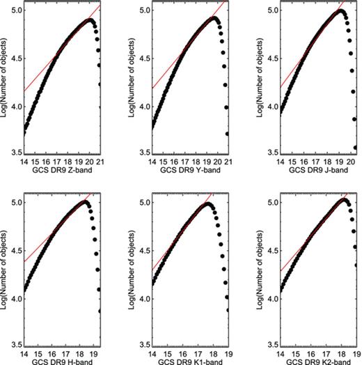
Completeness of the GCS DR9 data set in the α Per cluster in each of the six filters. The polynomial fit of order 2 is shown as a red line and defines the 100 per cent completeness limit of the GCS DR9 in each passband.

The query returned 2643 045 sources with J = 11.0–21.2 mag over ∼56 square degrees towards the α Per cluster. The full coverage is displayed in Fig. ⁰⁰⁰² and the resulting (Z − J,Z) colour–magnitude diagram is shown in Fig. ⁰⁰⁰³ along with previously published member candidates (black filled dots). Note that theoretical isochrones plotted in this paper were specifically computed for the WFCAM set of filters at an age of 90 Myr (downloaded from France Allard's webpage). We combined the NextGen and DUSTY isochrones for effective temperatures above and below 2700 K, respectively, to convert magnitudes into masses (Section ).

Figure 2

Open in new tabDownload slide

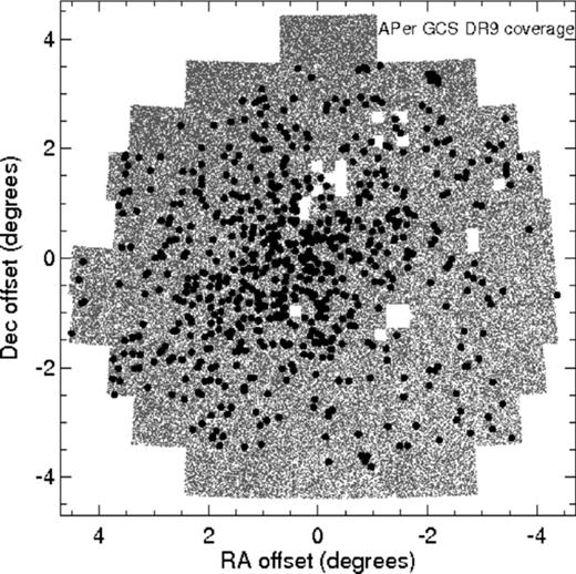
Coverage from the UKIDSS GCS DR9 in the α Per open cluster in the standard angular plane coordinates (ξ, η) choosing (RA, Dec.) = (51°, 49°) as the cluster centre. The total area covered is about 56 square degrees. The holes present in the coverage are due to the rejection of some tiles after quality control. GCS DR9 member candidates identified in this work are overplotted as black filled dots.

Figure 3

Open in new tabDownload slide

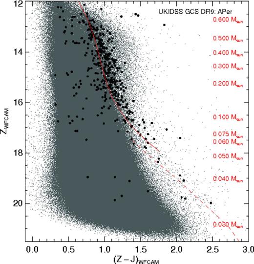
(Z − J, Z) CMD for ∼56 square degrees in the α Per extracted from the UKIDSS Galactic Cluster Survey Data Release 9. Previously published member candidates in α Per are overplotted as filled dots. The mass scale is shown on the right-hand side of the diagrams and extends down to 0.03 M_⊙, according to the NextGen and DUSTY models assuming an age of 90 Myr and a distance of 172.4 pc (Baraffe et al. ; Chabrier et al. ).

3 CROSS-MATCH WITH PREVIOUS SURVEYS

There are 455 probable members known in α Per extracted from previous proper motion and optical surveys (Heckmann et al. ; Mitchell ; Fresneau ; Stauffer et al. , , ; Prosser , ; Prosser & Randich ; Prosser et al. ; Barrado y Navascués et al. ; Lodieu et al. ), and an additional 300 high-probability (p ≥ 60 per cent) member candidates from Deacon & Hambly ().

We cross-matched catalogues from earlier studies with our full sample of over ∼2.5 million sources retrieved from GCS DR9 to locate the cluster sequence in various colour–magnitude diagrams. We recovered a total of 426 known members in α Per after removing multiple detections present in various catalogues (Table ⁰⁰⁰⁶). The numbers and percentages in brackets in the second and sixth column of Table ⁰⁰⁰¹ consider previously published sources lying in the magnitude range probed by the GCS. We also made a detailed analysis of the 629 previously known members not recovered by our SQL query. The numbers are given in the fourth column of Table ⁰⁰⁰⁶ which is divided into five sub-columns. Most of these sources are either missing an image in J, H or K1, are not covered by the GCS (223 or 35.5 per cent), are brighter than the saturation limits set in our query (205 or 32.6 per cent) or are very likely proper motion non-members (48 or 7.6 per cent).

4 NEW SUBSTELLAR MEMBERS IN α Per

4.1 Probabilistic approach

4.1.1. Method

In this section we outline the probabilistic approach we employed to select low-mass stars and brown dwarf member candidates in α Per using photometry and astrometry from the UKIDSS GCS DR9. This method is described in detail in Deacon & Hambly () and Lodieu et al. (). The main steps are as follows.

• Define the cluster sequence using candidates published in the literature within the area covered by the GCS DR9.

• Make a conservative cut in the (Z − J, Z) diagram to include known members and any new cluster member candidates defined as Z ≥ 16.5 and Z ≤ (11.5 + 5.0 × (Z − J)) OR Z ≤ 16.5 and Z ≤ (8.5 + 8.0× (Z − J)) displayed as solid black lines in the top-left panel of Fig. ⁰⁰⁰⁵.

• Analyse the vector point diagram in a probabilistic manner to assign a membership probability for each photometric candidate with a proper motion measurement (Section ).

• Derive the luminosity and mass function by summation of membership probabilities to provide a statistically complete sample.

Figure 4

Open in new tabDownload slide

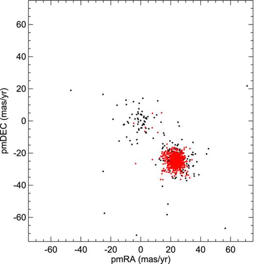
Vector point diagram showing the proper motion in right ascension (x axis) and declination (y axis) for previously known member candidates recovered by the GCS DR9 (black dots) and the new member candidates selected with method 2 (red dots).

Figure 5

Open in new tabDownload slide

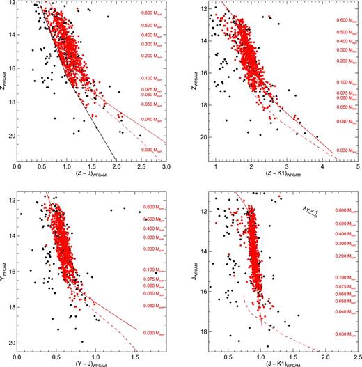
Colour–magnitude diagrams showing the member candidates previously reported in α Per (black dots) and all candidates extracted from our probabilistic analysis, including known ones (red dots). Upper-left: (Z − J, Z); upper-right: (Z − K, Z); lower-left: (Y − J, Y); lower-right: (J − K, J). Overplotted are the 90 Myr NextGen (solid line; Baraffe et al. ) and DUSTY (dashed line; Chabrier et al. ) isochrones shifted to a distance of 120 pc. The mass scale is shown on the right-hand side of the diagrams and spans 0.60–0.03 M_⊙, according to the 90 Myr isochrone models. The solid black lines in the upper-left diagram represent our conservative photometric cuts used for the probabilistic approach.

4.1.2. Membership probabilities

In order to calculate formal membership probabilities we have used the same technique as in Lodieu et al. () to fit distribution functions to proper motion vector point diagrams (Hambly et al. ). The technique differs slightly from the original method presented in Deacon & Hambly () and Lodieu et al. () in that the value of sigma (σ) is fixed by the formal astrometric errors propagated from the centroiding errors given by the source extraction software employed upstream of the WFCAM Science Archive (Hambly et al. ), the main repository of UKIDSS data.

We refer the reader to the above-cited papers for more details and additional equations. First, we rotate the vector point diagram so that the cluster lies on the y axis, assuming a proper motion of (22.73,−26.51) mas yr⁻¹ for α Per (van Leeuwen ) after applying a very conservative photometric selection in the (Z − J,Z) colour–magnitude diagram. We also note that we used the following rotation for the vector point diagram:

• = cos (0.77 × PI) × μ_x − sin (0.77 × PI) × μ_y

• = cos (0.77 × PI) × μ_x + sin (0.77 × PI) × μ_y.

We have assumed that there are two contributions to the total distribution φ(μ_x, μ_y), one from the cluster, 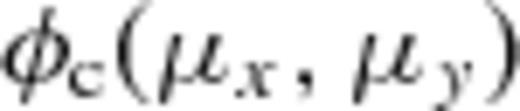, and one from the field stars, . The fitting region was delineated by −50 < μ_x < 50 mas yr⁻¹ and −50 < μ_y < 50 mas yr⁻¹. These were added by means of a field star fraction f.

We characterized the cluster distribution as a bivariate Gaussian with a single standard deviation σ and mean proper motion values in each axis μ_xc and μ_yc. The field star distribution was fitted by a univariate Gaussian in the x axis (with standard deviation Σ_x and mean ) and a declining exponential in the y axis with a scale length τ. The use of a declining exponential is a standard method (e.g. Jones & Stauffer ) and is justified in that the field star distribution is not simply a circularly symmetric error distribution (i.e. capable of being modelled as a 2D Gaussian) – rather there is a preferred direction of real field star motions resulting in a characteristic velocity ellipsoidal signature, i.e. a non-Gaussian tail, in the vector point diagram. This is best modelled (away from the central error-dominated distribution) as an exponential in the direction of the antapex (of the solar motion).

The best-fitting set of parameters were chosen using a maximum likelihood method (see Deacon & Hambly ). However in a deviation from this method we did not fit for the standard deviation of the cluster proper motions (σ). Instead we calculated the mean astrometric error for all objects in each magnitude range and used this as our cluster standard deviation. This fitting process was tested by Deacon & Hambly () where simulated data sets were created and run through the fitting process to recover the input parameters. These tests produced no significant offsets in the parameter values (see table 3 and appendix A of Deacon & Hambly , for results and more details on the procedure). Hence, we calculated the formal membership probabilities as

1

 We split the sample into eight intervals of magnitudes because astrometric errors are a function of magnitude and also to improve the contrast between the field stars and the cluster. Each band is one magnitude wide and was fitted with all seven parameters in the same way as described in Deacon & Hambly (). There was no fit possible for the 20–21 magnitude bins because of the small number of sources in this bin. A summary of the fitted parameters from the probabilistic analysis described above is given in Table ⁰⁰⁰².

Table 2

Summary of the results after running the program to derive membership probabilities. For each Z magnitude range, we list the number of stars used in the fit (Nb), the field star fraction f and parameters describing the cluster and field star distribution. Units are in mas yr⁻¹ except for the number of stars and the field star fraction f. The cluster star distribution is described by the mean proper motions in the x and y directions ( and ) and a standard deviation σ. Similarly, the field star distribution is characterized by a scale length for the y axis (τ), a standard deviation Σ_x and a mean proper motion in the x direction (). Note that the value of sigma (σ) is fixed by the formal astrometric errors

Z	Nb	f	σ			τ	Σx
12–13	206	0.84	2.84	−1.64	33.24	16.56	21.67	4.76
13–14	488	0.75	2.82	−1.98	33.91	21.32	16.27	0.78
14–15	720	0.77	2.78	−1.73	33.99	16.83	16.21	0.60
15–16	913	0.83	2.85	−1.74	33.47	14.69	15.05	−0.50
16–17	877	0.86	2.88	−2.15	34.30	14.68	14.66	0.21
17–18	503	0.92	3.05	−1.42	33.35	13.71	14.27	0.08
18–19	224	0.89	3.52	−2.39	31.24	17.35	15.38	0.98
19–20	203	0.90	5.12	−3.12	31.62	12.39	14.81	−0.39

Z	Nb	f	σ			τ	Σx
12–13	206	0.84	2.84	−1.64	33.24	16.56	21.67	4.76
13–14	488	0.75	2.82	−1.98	33.91	21.32	16.27	0.78
14–15	720	0.77	2.78	−1.73	33.99	16.83	16.21	0.60
15–16	913	0.83	2.85	−1.74	33.47	14.69	15.05	−0.50
16–17	877	0.86	2.88	−2.15	34.30	14.68	14.66	0.21
17–18	503	0.92	3.05	−1.42	33.35	13.71	14.27	0.08
18–19	224	0.89	3.52	−2.39	31.24	17.35	15.38	0.98
19–20	203	0.90	5.12	−3.12	31.62	12.39	14.81	−0.39

Open in new tab

Table 2

Summary of the results after running the program to derive membership probabilities. For each Z magnitude range, we list the number of stars used in the fit (Nb), the field star fraction f and parameters describing the cluster and field star distribution. Units are in mas yr⁻¹ except for the number of stars and the field star fraction f. The cluster star distribution is described by the mean proper motions in the x and y directions ( and ) and a standard deviation σ. Similarly, the field star distribution is characterized by a scale length for the y axis (τ), a standard deviation Σ_x and a mean proper motion in the x direction (). Note that the value of sigma (σ) is fixed by the formal astrometric errors

Z	Nb	f	σ			τ	Σx
12–13	206	0.84	2.84	−1.64	33.24	16.56	21.67	4.76
13–14	488	0.75	2.82	−1.98	33.91	21.32	16.27	0.78
14–15	720	0.77	2.78	−1.73	33.99	16.83	16.21	0.60
15–16	913	0.83	2.85	−1.74	33.47	14.69	15.05	−0.50
16–17	877	0.86	2.88	−2.15	34.30	14.68	14.66	0.21
17–18	503	0.92	3.05	−1.42	33.35	13.71	14.27	0.08
18–19	224	0.89	3.52	−2.39	31.24	17.35	15.38	0.98
19–20	203	0.90	5.12	−3.12	31.62	12.39	14.81	−0.39

Z	Nb	f	σ			τ	Σx
12–13	206	0.84	2.84	−1.64	33.24	16.56	21.67	4.76
13–14	488	0.75	2.82	−1.98	33.91	21.32	16.27	0.78
14–15	720	0.77	2.78	−1.73	33.99	16.83	16.21	0.60
15–16	913	0.83	2.85	−1.74	33.47	14.69	15.05	−0.50
16–17	877	0.86	2.88	−2.15	34.30	14.68	14.66	0.21
17–18	503	0.92	3.05	−1.42	33.35	13.71	14.27	0.08
18–19	224	0.89	3.52	−2.39	31.24	17.35	15.38	0.98
19–20	203	0.90	5.12	−3.12	31.62	12.39	14.81	−0.39

Open in new tab

4.1.3. Probabilistic sample

The probabilistic approach yielded a total sample of 10 176 sources with membership probabilities assigned to each of them. This sample contains 728 sources with membership probabilities higher than 40 per cent (including known ones previously published) listed in Table ⁰⁰⁰⁷. Tightening this probability threshold to 50 and 60 per cent yields samples of 573 (∼27 per cent less) and 431 (∼69 per cent less) member candidates in α Per, respectively. These high-probability members are displayed in Fig. ⁰⁰⁰⁵ with previously published candidates in α Per plotted in black.

4.2 Photometry and proper motion selection

In this section we outline a more widely used method (referred to as method 2 in the rest of the paper) that we applied to select low-mass and substellar member candidates in α Per. This procedure consists of selecting cluster candidates by applying proper motion selection followed by strict photometric cuts in various colour–magnitude diagrams. This alternative method provides an independent test of the probabilistic approach presented in the previous section.

The first step was to select all sources with formal errors on the proper motion within 3σ of the mean proper motion of the cluster (Fig. ⁰⁰⁰⁴), yielding a completeness better than 99 per cent assuming normally distributed errors. The main advantage of this method is that it does not rely on a single radius for the proper motion selection but rather takes into account the increasing uncertainty on the proper motion measurements between the GCS epochs with decreasing brightness.

Secondly, we plotted several colour–magnitude diagrams (Fig. ⁰⁰⁰⁵) to define a series of lines based on the position of known α Per members identified in earlier studies and published over the past decades (Table ⁰⁰⁰¹). Those lines detailed below are plotted in Fig. ⁰⁰⁰⁶ and improve on the pure proper motion selection. We note that those criteria are similar to those used for the Pleiades (Lodieu et al. ) because the younger age of α Per compared to the Pleiades is compensated by its larger distance.

• (Z − J, Z) = (0.60,12.0) to (1.20,16.5)

• (Z − J, Z) = (1.20,16.5) to (2.00,20.0)

• (Z − K, Z) = (1.20,11.5) to (1.95,17.0)

• (Z − K, Z) = (1.95,17.0) to (4.00,21.5)

• (Y − J, Y) = (0.30,11.5) to (0.55,16.5)

• (Y − J, Y) = (0.55,16.0) to (1.40,20.5)

• (J − K, J) = (0.75,11.0) to (0.75,16.5)

• (J − K, J) = (0.75,16.5) to (1.70,19.0).

Figure 6

Open in new tabDownload slide

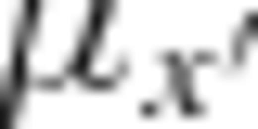
Same as Fig. ⁰⁰⁰⁵ but only for member candidates in α Per selected using method 2. The Y JHK- and JHK-only detections have been added too for completeness.

This selection returned a total of 685 low-mass stars and brown dwarfs with Z magnitude ranging from 12 to 21.5, including known ones recovered by the GCS (Table ⁰⁰⁰⁸). This total number is similar to the number of high-probability member candidates – 728 (431) with p > 40 (60) per cent – in α Per identified via the probabilistic approach.

4.3 Search for lower mass members

In this section we search for fainter and cooler substellar members in α Per by dropping the constraint on the Z-band detection and later the Z + Y bands.

4.3.1. Y JHK detections

To extend the α Per cluster sequence to fainter brown dwarfs and cooler temperatures, we searched for potential candidate members undetected in Z. We imposed similar photometric and astrometric criteria as those detailed in Section but analysed Z drop-outs as follows:

• Y ≥ 18 and J ≤ 19.1 mag.

• Candidates should lie above the line defined by (Y − J, Y) = (0.55,16.0) and (1.40,20.5).

• Candidates should lie above the line defined by (J − K, J) = (0.75,16.5) and (1.70,19.0).

• The position on the proper motion vector point diagram of each candidate should not deviate from the assumed cluster proper motion by more than 3σ.

This selection returned 13 additional member candidates in α Per (Table ⁰⁰⁰⁹). All but four of them are indeed undetected in the Z-band images and look well detected in the other bands after checking the GCS DR9 images. Thus we are left with nine bona-fide member candidates.

4.3.2. JHK detections

We repeated the procedure described above looking for Z and Y non-detections. We additionally applied the following criteria:

• J = 18–19.1 mag.

• Candidates should lie above the line defined by (J − K, J) = (0.75,16.5) and (1.70,19.0).

• The position on the proper motion vector point diagram of each candidate should not deviate from the assumed cluster proper motion by more than 3σ.

This query returned 36 new candidate members in α Per. After checking the GCS images, we retained only eight of them as bona-fide candidates because the others actually appear in the Z and/or Y images (although detections are not reported in the GCS DR9 catalogue) or have no Z and/or Y images. The reasons for the rejection of 28 of the 36 candidates is given in the last column of Table ⁰⁰⁰⁹.

5 ESTIMATION OF THE CONTAMINATION

In this section we estimate the level contamination present in our photometric and astrometric selection (method 2).

The number density of field objects in our final list of candidates as a function of mass is obtained in a similar way as in Boudreault et al. (). We obtained the radial profile of our cluster candidates in three mass ranges: above 0.3 M_⊙, between 0.072 and 0.3 M_⊙ and below the hydrogen-burning limit at 0.072 M_⊙ (Fig. ⁰⁰⁰⁸).

Figure 7

Open in new tabDownload slide

Difference in the K magnitude (K1–K2) as a function of the K1 magnitude for all member candidates in α Per selected with method 2. The Y JHK- and JHK-only detections have been added too (dots with open squares and open triangles, respectively). Typical error bars on the K1–K2 colours as a function of magnitude are displayed as dotted lines.

Figure 8

Open in new tabDownload slide

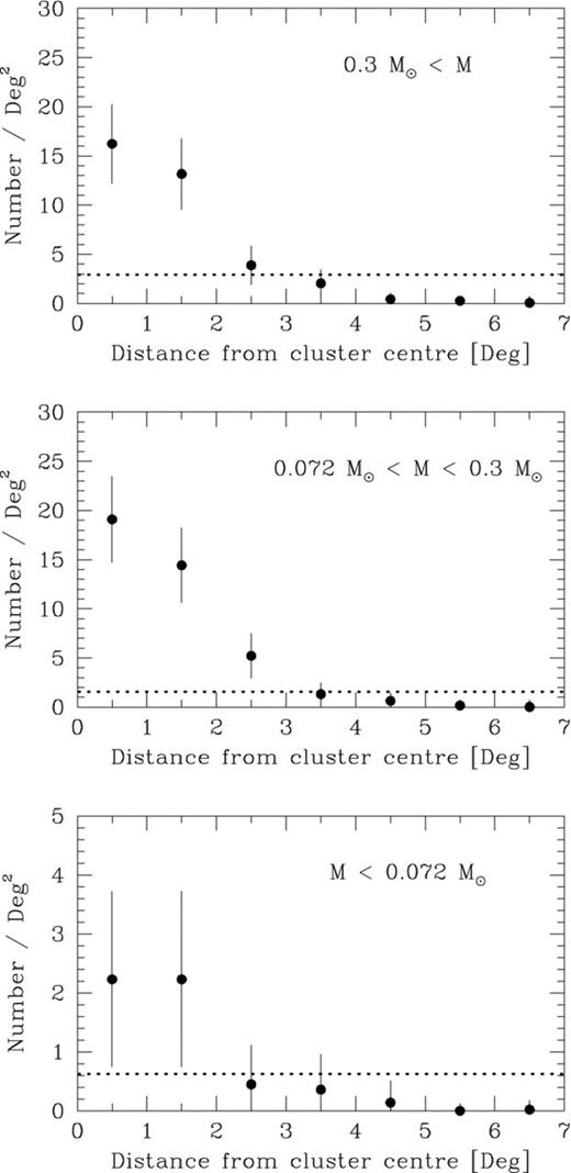
Radial density plots of our candidate members of α Per in three mass ranges: above 0.3 M_⊙ (top panel), between 0.72 and 0.3 M_⊙ (middle panel) and below the stellar/substellar limit at 0.072 M_⊙ (bottom panel). The error bars on each data point are Poissonian arising from the number of objects in each bin. The dotted horizontal line is the estimated contamination per square degree for each mass range.

However, considering the incomplete coverage of the UKIDSS GCS DR9 towards α Per (holes present in the coverage due to quality control, see Fig. ⁰⁰⁰²), all data points must be considered as lower limits: we are only partly complete up to the tidal radius of α Per at 2°.91 (9.7 pc; Makarov ) and up to 3°.5 (95 per cent complete in coverage). Consequently, the estimated contamination represents an upper limit.

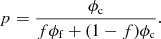
We used only the number of objects between 3° and 3°.5 (outside the estimated tidal radius) at each mass range to obtain an upper limit of contamination. This gives 2.92 objects per square degree for candidates with masses above 0.3 M_⊙, 1.57 between 0.072 and 0.3 M_⊙ and 0.62 objects per square degree for our substellar candidates. Within 3° from the cluster centre, this gives a contamination of 35.1, 15.9 and 50.6 per cent for the same mass range, respectively, or 26.3 per cent for the whole α Per sample within 3°. This level of contamination brings into agreement within a factor of 2 the luminosity functions derived from both selection methods highlighted in this paper (left-hand side panel of Fig. ⁰⁰⁰⁹).

Figure 9

Open in new tabDownload slide

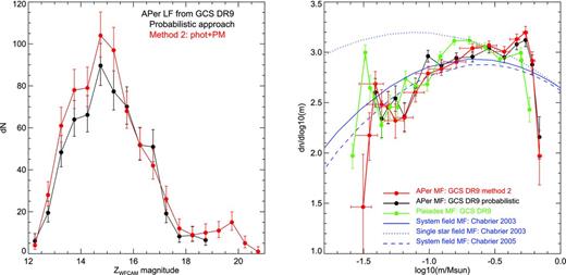
Luminosity (left) and system mass (right) functions derived from our analysis of the UKIDSS GCS DR9 sample of member candidates in α Per. Error bars are Gehrels errors. The brightest bin and the last bins are very likely contaminated because of saturation and incompleteness, respectively. The left-hand side panel compares the luminosity function obtained from the probabilistic approach (black symbols and black line) and the luminosity function derived from the selection outlined by method 2 (red colour). Note that the sample of method 2 extends two magnitude bins fainter but they are incomplete as is the brightest bin due to saturation. The right-hand side panel compares the α Per mass function derived from this probabilistic approach (filled black dots linked by a solid line) and the mass function derived from method 2 (red symbols and red line). Error bars on the mass (x axis) are 3σ uncertainties considering the errors on the age and distance of α Per. The Pleiades mass function derived in a similar manner is overplotted in green for comparison along with the field (system) mass functions in blue (Chabrier ).

These numbers appear quite large. We stress again that these are upper limits, since the coverage is not complete. However, we can claim the completeness higher than 90 per cent for our cluster candidate list and the determination of our mass function. This is justified by the fact that our astrometric selection includes all objects within 3σ of the cluster's mean proper motion (completeness of >99 per cent) and that the lines used in our photometric selection go at least 2σ bluer from the cluster main sequence in all the colour–magnitude diagrams used for the photometric selection (completeness of ∼95.4 per cent).

Most of the contaminants of our cluster candidates with masses above 0.1 M_⊙ would be Galactic disc late-type and giant stars, while most of the contaminants of candidates less massive than 0.1 M_⊙ would include Galactic disc late-type and giant stars, but also unresolved galaxies.

6 VARIABILITY AT 90 Myr

In this section we discuss the K-band variability of the low-mass stars and brown dwarfs in α Per using the two epochs provided by the GCS. First we considered the candidates extracted with method 2, several of them being already published in the literature (Tables ⁰⁰⁰⁶).

Fig. ⁰⁰⁰⁷ shows (K1–K2) versus K1 for all candidate members in α Per from method 2. The brightening in the K1 = 11–12 mag range is due to the difference in depth between the first and second epoch, around 0.5 mag both in the saturation and completeness limit. This is understandable because the exposure times have been doubled for the second epoch with relaxed constraints on the seeing requirement and weather conditions. We excluded those objects from our variability study. Overall, the sequence is very well defined and very few objects appear variable in the K band.

We selected variable objects by looking at the standard deviation, robustly estimated as 1.48× the median absolute deviation which is the median of the sorted set of absolute values of deviation from the central value of the K1–K2 colour. We identified one potential variable object in the K1 = 11–12 and 12–13 mag range with differences in the K band larger than 3σ above the standard deviation. No additional variable source was picked up beyond 3σ down to K1 = 16.5 mag. The candidate selected in the brightest bin appears saturated in the second epoch image, suggesting that the variability may be caused by the inaccurate photometry derived from saturated sources. The other source does not look saturated: its variability may be attributed to the presence of a faint companion located south-east at ∼1.2 arcsec best visible in the K2 image due to the greater depth of the second epoch. This variability analysis is not feasible for K1 ≥ 16.5 mag due to the small number of α Per candidate members beyond that magnitude range.

We conclude that the level of variability at 90 Myr is small, with standard deviations in the 0.06–0.09 mag range, suggesting that it cannot account for the dispersion in the cluster sequence. The same conclusions are drawn from the high-probability sample and are consistent with our analysis of the Pleiades (Lodieu et al. ) and Praesepe (Boudreault et al. ) samples although we should point out that a handful of members are found to be variable.

7 THE LUMINOSITY AND INITIAL MASS FUNCTIONS

In this section we discuss the cluster luminosity and mass functions derived from the samples of member candidates in α Per extracted from both methods described in the previous section. We did not attempt to correct the mass function for binaries; hence, we compare our results to ‘system’ mass functions. Note that contrary to our work in the Pleiades and Praesepe, we are unable to estimate the substellar multiplicity due to larger scatter in the single-star and binary sequences due to crowding.

7.1 Age and distance of α Per

Age determinations in open clusters can vary by up to a factor of 2 (Jeffries & Naylor ): fitting of the upper main-sequence and giant branch (Mermilliod ) comparing with models including some convective overshoot (Maeder & Mermilliod ) tend to yield younger ages than the lithium test (Rebolo, Martín & Magazzù ). In the case of α Per, the former method gives 51 Myr whereas the latter suggests an age between 85 ± 10 (Barrado y Navascués, Stauffer & Jayawardhana ) and 90 ± 10 Myr (Stauffer et al. ). A similar discrepancy has been observed for the Pleiades (77 Myr versus 120 Myr; Mermilliod ; Stauffer, Schultz & Kirkpatrick ). Moreover, Meynet, Mermilliod & Maeder () revised the ages of 30 galactic open clusters based on an updated set of solar-metallicity isochrones (at that time) taking into account mass loss and moderate overshooting, yielding 52 and 100 Myr for the α Per and the Pleiades, respectively. The latter age for the Pleiades is favoured by the fitting technique of the main-sequence evolution developed by Naylor () which quoted a 68 per cent confidence interval of 104–117 Myr (mean value of 115 Myr), in agreement with the careful comparison of model isochrones to the Pleiades photometric sequence by Bell et al. (). Other clusters with ages derived by the lithium depletion boundary tend to agree with older age estimates although with a possible trend towards slightly older ages, e.g. IC 4665 (36 Myr versus 28 ± 4 Myr Mermilliod ; Manzi et al. ), IC 2602 (30–67 Myr versus 46 ± 6 Myr; Kharchenko et al. ; Dobbie, Lodieu & Sharp ), NGC 2547 (20–35 Myr versus 34–36 Myr; Naylor et al. ; Jeffries & Oliveira ) or M35 (200 Myr versus 175 Myr; Sung & Bessell ; Barrado y Navascués, Deliyannis & Stauffer ). We will employ the isochrones for the lithium test age of 90 Myr in the case of α Per, bearing in mind the current uncertainty on its age of the order of 10 Myr.

Several distance estimates have been published for α Per: 190.5 pc by Robichon et al. (), 176.2  ±  5.0 pc by Pinsonneault et al. () and Makarov (). The latest value derived from a revised reduction of the Hipparcos data by van Leeuwen () suggests a distance of 172.4 ± 2.7 pc which we adopt in this work.

To summarize, we adopt in this work a distance of 172.4 pc (van Leeuwen ) and employed the Lyon group NextGen (Baraffe et al. ) and DUSTY (Chabrier et al. ) models at an age of 90 Myr to convert the luminosity function into a mass function. We should point out that the lowest mass brown dwarfs in α Per are warmer than 1400 K, the upper limit where the COND models should be used (Baraffe et al. ).

7.2 The luminosity function

In this section, we construct two luminosity functions: (i) we used the sample of 10 176 stars in α Per with computed membership probabilities (Section ) and (ii) the 685 candidates identified with method 2 (Section ). The luminosity function of the former method is derived by summing membership probabilities of all stars fitted to distribution functions in the vector point diagram, whereas the luminosity function of the latter is derived simply by summing the number of member candidates.

Both luminosity functions, i.e. the number of stars and brown dwarfs as a function of magnitude plotted per 0.5 mag bin, are displayed in Fig. ⁰⁰⁰⁹. Both luminosity functions look very similar and match each other within the error bars. The numbers of objects per 0.5 mag bin increase quickly to reach a peak around Z = 14.5–15 and drop off afterwards down to the completeness of our survey with a possible peak around Z = 19.5–20 mag (Tables ⁰⁰⁰³ and ⁰⁰⁰⁴). The brightest bin is a lower limit due to the saturation limit of the GCS survey. The last four bins included in method 2 are not present in the probabilistic approach because the broad cluster distribution and low separation from the field causes the probabilities to be washed out. All bins in the probabilistic luminosity function are complete while the last two bins from method 2 are incomplete due to the constraints imposed on the Z-band detection. Moreover, the α Per luminosity function is very similar to the Pleiades one derived in a similar manner using the same homogeneous survey (Lodieu et al. ) although less populated mainly because of the smaller areal coverage.

7.3 The mass function

In this section we adopt the logarithmic form of the IMF as originally proposed by Salpeter (): ξ(log₁₀ m) = dn / d log₁₀(m) ∝ m^−x where the exponent of the mass spectrum α = x + 1 following the formulation of Chabrier (). The Z = 12–21 mag range translates into masses between ∼0.74 and ∼ 0.03 M_⊙ (19 mag and 0.046 M_⊙ in the case of the probabilistic approach), assuming a revised distance of 172.4 pc (van Leeuwen ) and an age of 90 Myr for which the models are computed.

We included in Fig. ⁰⁰⁰⁹ errors in both the x axis (log M) and y axis (dN/d log M) as follows. For the error bars on the masses, we considered three times the uncertainties on the age (90 ± 10 Myr; Stauffer et al. ) and distance (172.4 ± 2.7 pc; van Leeuwen ) of α Per given us a validity range of 3 σ on the x axis. Hence, we computed the masses with the 60 Myr NextGen and DUSTY isochrones shifted at a distance of 164.3 pc to define the lower limit and repeated the procedure with the 120 Myr isochrones for a distance of 180.5 pc as upper limits. The uncertainties on the y axis, i.e. the dN/d log M values, are simply Gehrels error bars. This α Per mass function, directly compared to the Pleiades (Lodieu et al. ) and the field (Chabrier ) mass functions, agree within the error bars. We should point out the recent mass function of the field published by Kroupa et al. () and described as a power law is almost identical to the log-normal form of Chabrier ().

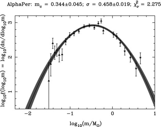
In Fig. ⁰⁰¹⁰ we show a log-normal fit for α Per incorporating higher mass data points from Prosser () in order to provide constraint on the parameters of the fit, in particular the characteristic mass which requires sufficient points on both sides of the peak in the function. We translated the ‘corrected’ luminosity function values making a small update to the absolute magnitudes for the distance modulus used here (6.18) over the value of 6.1 in Prosser (). The visual band mass–luminosity relation used comes from Marigo et al. () evolutionary models. We include in the fit only those higher mass points that are complete, i.e. for M_V < +5 from Prosser (), and excluding our own highest mass point from the GCS luminosity function, but we include the four lowest mass points from the GCS since excluding them does not significantly alter the fit. The mass function appears to be well represented by a log-normal with goodness of fit which indicates some systematic fluctuations over and above the assumed sampling errors that could easily be due to sample contamination and/or systematic errors resulting from the assumed models.

Figure 10

Open in new tabDownload slide

Log-normal fit to the GCS DR9 data (method 2; triangles with error bars) in conjunction with higher mass data points (stars with error bars) taken from Prosser (). The least-squares fit to the data points is the solid line with the shaded region corresponding to a formal 1σ uncertainty.

It is interesting to compare this mass function with those from the Pleiades (Lodieu et al. ) and Praesepe (Boudreault et al. ), with similar higher mass constraints from optical photographic plate surveys – see Fig. ⁰⁰¹¹. In the case of the Pleiades and α Per, the higher mass luminosity functions have been taken as complete and no normalization has been performed relative to the GCS luminosity functions, whereas for Praesepe we found that the mass function resulting from the Jones & Stauffer () luminosity function is discontinuous with the GCS mass function from Boudreault et al. (). We determined a relative normalization of 0.447 in the log (a factor 2.8) for a minimal chi-squared in the log-normal fit for Praesepe.

Figure 11

Open in new tabDownload slide

Log-normal fit to the GCS DR9 data (triangles with error bars) in conjunction with higher mass data points (stars with error bars) taken for the Pleiades [Lodieu, Deacon & Hambly , excluding the three lowest mass bins; higher mass points from the unpublished compilations of Prosser and Stauffer, see for example Hambly et al. () and references therein]; α Per (this work) and Praesepe [Boudreault et al. (); higher mass points from Jones & Stauffer ()]. In each case, least-squares fits to the data points are the solid line with the shaded region corresponding to a formal 1σ uncertainty.

In Table ⁰⁰⁰⁵ we compare the log-normal fit parameters to the field system mass function parametrized by Chabrier (, ). There is some marginal evidence here for a variation in characteristic mass at the 1 to 2σ level between α Per and Praesepe and the Pleiades, but this must be treated with caution given the range of goodness of fits obtained () and particularly the significant departure from the fit for the Pleiades at the low-mass end. There is a clear statistically significant difference between the dispersion values of the field and α Per mass functions, not unexpected due to the difference in age. While we caution that the fitted values can be sensitive to the relative normalization between the GCS and higher mass data, changes in the relative offsets tend to narrow the log-normal fit rather than broaden it. In any case, it is interesting to note the general log-normal trend in these wide mass range mass functions.

Table 5

Comparison between log-normal mass function parameters for the α Per, Pleiades and Praesepe clusters as determined from GCS DR9 data in conjunction with higher mass bin data from optical photographic proper motion surveys, compared with the field system mass function parameters quoted by Chabrier (, )

Population	Characteristic	Dispersion
	mass mC (M⊙)	σ
α Per	0.344 ± 0.045	0.458 ± 0.019	2.275
Pleiades	0.247 ± 0.047	0.456 ± 0.023	4.382
Praesepe	0.328 ± 0.035	0.434 ± 0.015	0.962
Field (Chabrier )	0.22	0.57
Field (Chabrier )	0.25	0.55

Population	Characteristic	Dispersion
	mass mC (M⊙)	σ
α Per	0.344 ± 0.045	0.458 ± 0.019	2.275
Pleiades	0.247 ± 0.047	0.456 ± 0.023	4.382
Praesepe	0.328 ± 0.035	0.434 ± 0.015	0.962
Field (Chabrier )	0.22	0.57
Field (Chabrier )	0.25	0.55

Open in new tab

Table 5

Comparison between log-normal mass function parameters for the α Per, Pleiades and Praesepe clusters as determined from GCS DR9 data in conjunction with higher mass bin data from optical photographic proper motion surveys, compared with the field system mass function parameters quoted by Chabrier (, )

Population	Characteristic	Dispersion
	mass mC (M⊙)	σ
α Per	0.344 ± 0.045	0.458 ± 0.019	2.275
Pleiades	0.247 ± 0.047	0.456 ± 0.023	4.382
Praesepe	0.328 ± 0.035	0.434 ± 0.015	0.962
Field (Chabrier )	0.22	0.57
Field (Chabrier )	0.25	0.55

Population	Characteristic	Dispersion
	mass mC (M⊙)	σ
α Per	0.344 ± 0.045	0.458 ± 0.019	2.275
Pleiades	0.247 ± 0.047	0.456 ± 0.023	4.382
Praesepe	0.328 ± 0.035	0.434 ± 0.015	0.962
Field (Chabrier )	0.22	0.57
Field (Chabrier )	0.25	0.55

Open in new tab

Assuming that the observed lithium depletion boundary is at M ∼ 0.075 M_⊙ (M_Z = 11.155; Stauffer et al. ; Barrado y Navascués et al. ) and a distance of 172.4 pc, the sample extracted by method 2 contains 685 α Per member candidates, divided up into 632 stars (92.3 per cent) and 53 brown dwarfs (7.7 per cent). Lower percentages of brown dwarfs are obtained considering the sample of 431–728 high-probability members (p ≥ 40–60 per cent) identified in the probabilistic approach, because of larger uncertainties on the probabilities at the faint end. Hence, the star (∼0.6–0.08 M_⊙) to brown dwarf (0.08–0.04 M_⊙) ratio in α Per spans 11.9 (10.4–12.7; 3σ limits using the lower and upper distance estimates) to 16.8–33.3, in agreement with measurements in IC 348 (8.3–11.6; Luhman et al. ; Andersen et al. ) but higher than other open clusters like M35 (4.5; Barrado y Navascués et al. ) or the Pleiades (3.7 and 5.7–8.8; Bouvier et al. ; Lodieu et al. ), young star-forming regions (3.0–6.4 for the Trapezium Cluster; 3.8–4.3 for σ Orionis; 3.8 for Chamaeleon; Hillenbrand & Carpenter ; Muench et al. ; Andersen et al. ; Luhman ; Lodieu et al. ), the field (1.7–5.3; Kroupa ; Chabrier ; Andersen et al. ) and hydrodynamical simulations of star clusters (3.8–5.0; Bate , ). We list the ranges of the ratios because the stellar and substellar intervals differ slightly from study to study.

8 SUMMARY

We have presented the outcome of a wide (∼56 square degrees) and deep (J ∼ 19.1 mag) survey in the α Per open cluster as part of the UKIDSS GCS DR9. The main results of our study can be summarized as follows.

• We recovered member candidates in α Per previously published and updated their membership assignations.

• We selected photometrically and astrometrically potential α Per member candidates using two independent but complementary methods: the probabilistic analysis and a more standard method combining photometry and proper motion cuts.

• We investigated the K-band variability of α Per cluster members and found virtually no variability at the level of 0.06–0.09 mag.

• We derived the luminosity function from both selection methods and found no difference within the error bars.

• We derived the α Per mass function over the 0.5–0.04 M_⊙ mass range: its shape is similar to the Pleiades mass function and best represented by a log-normal form with a characteristic mass of 0.34 M_⊙ and a dispersion of 0.46.

This paper represents a significant improvement in our census of the α Per low-mass and substellar population as well as our knowledge of the mass function across the hydrogen-burning limit over the entire cluster. We believe that this paper will represent a reference for many more years to come in α Per. We will now extend this study to other regions surveyed by the GCS to address the question of the universality of the mass function using a homogeneous set of photometric and astrometric data. Future work to constrain current models of star formation includes the search for companions to investigate their multiplicity properties, the determination of the radial velocities of α Per members and deeper surveys to test the theory of the fragmentation limit.

NL is funded by the Ramón y Cajal fellowship number 08-303-01-02 and the national programme AYA2010-19136 funded by the Spanish Ministry of Science and Innovation (SB is also funded by this grant). We thank the referee, Tim Naylor, for his careful review and for advice concerning cluster age determinations which has led to an improved paper. This work is based in part on data obtained as part of the UKIRT Infrared Deep Sky Survey (UKIDSS). The UKIDSS project is defined in Lawrence et al. (). UKIDSS uses the UKIRT WFCAM (Casali et al. ). The photometric system is described in Hewett et al. (), and the calibration is described in Hodgkin et al. (). The pipeline processing and science archive are described in Irwin et al. (in preparation) and Hambly et al. (), respectively. We thank our colleagues at the UK Astronomy Technology Centre, the Joint Astronomy Centre in Hawaii, the Cambridge Astronomical Survey and Edinburgh Wide Field Astronomy Units for building and operating WFCAM and its associated data flow system. We are grateful to France Allard's homepage that we used to download the NextGen and DUSTY isochrones at 60, 90 and 120 Myr for the WFCAM filters.

This research has made use of the Simbad data base, operated at the Centre de Données Astronomiques de Strasbourg (CDS) and of NASA's Astrophysics Data System Bibliographic Services (ADS). This publication has also made use of data products from the Two Micron All Sky Survey, which is a joint project of the University of Massachusetts and the Infrared Processing and Analysis Center/California Institute of Technology, funded by the National Aeronautics and Space Administration and the National Science Foundation.

REFERENCES

Appendix A

TABLE OF KNOWN MEMBER CANDIDATES PREVIOUSLY PUBLISHED IN α Per AND RECOVERED IN the UKIDSS GCS DR9

Table A1

Sample of known member candidates previously published in α Per and recovered in GCS DR9. We list the equatorial coordinates (J2000), GCS ZY JHK1K2 photometry, proper motions (in mas yr⁻¹) and their errors, reduced chi-squared statistic of the astrometric fit for each source (χ² value), membership probabilities when available from our probabilistic study, and names from the literature. A ‘–’ in the probability column means that the object lacks measurement α Per member candidates are ordered by increasing right ascension. This table is available electronically as Supporting Information with the online version of the journal

RA	Dec.	Z	Y	J	H	K1	K2	±  err	μδ  ±  err	χ2	Prob	Name
02 58 17.66	+48 28 00.4	16.152	15.700	15.071	14.531	14.187	14.175	23.07 ± 2.91	−14.86 ± 2.91	0.59	–	DH12_Prob73.7
03 01 21.38	+48 35 23.3	13.971	13.664	13.142	12.494	12.257	12.267	24.39 ± 2.86	−21.71 ± 2.86	0.11	0.77	DH15_Prob70.8
…	…	…	…	…	…	…	…	…	…	…	…	…
03 50 37.08	+48 12 31.4	14.124	13.621	13.079	12.534	12.234	12.226	21.45 ± 2.03	−35.54 ± 2.03	6.38	–	AP265_M9.9_Y?
03 50 37.08	+48 12 31.4	14.124	13.621	13.079	12.534	12.234	12.226	21.45 ± 2.03	−35.54 ± 2.03	6.38	–	DH302_Prob79.1

RA	Dec.	Z	Y	J	H	K1	K2	±  err	μδ  ±  err	χ2	Prob	Name
02 58 17.66	+48 28 00.4	16.152	15.700	15.071	14.531	14.187	14.175	23.07 ± 2.91	−14.86 ± 2.91	0.59	–	DH12_Prob73.7
03 01 21.38	+48 35 23.3	13.971	13.664	13.142	12.494	12.257	12.267	24.39 ± 2.86	−21.71 ± 2.86	0.11	0.77	DH15_Prob70.8
…	…	…	…	…	…	…	…	…	…	…	…	…
03 50 37.08	+48 12 31.4	14.124	13.621	13.079	12.534	12.234	12.226	21.45 ± 2.03	−35.54 ± 2.03	6.38	–	AP265_M9.9_Y?
03 50 37.08	+48 12 31.4	14.124	13.621	13.079	12.534	12.234	12.226	21.45 ± 2.03	−35.54 ± 2.03	6.38	–	DH302_Prob79.1

Open in new tab

Table A1

Sample of known member candidates previously published in α Per and recovered in GCS DR9. We list the equatorial coordinates (J2000), GCS ZY JHK1K2 photometry, proper motions (in mas yr⁻¹) and their errors, reduced chi-squared statistic of the astrometric fit for each source (χ² value), membership probabilities when available from our probabilistic study, and names from the literature. A ‘–’ in the probability column means that the object lacks measurement α Per member candidates are ordered by increasing right ascension. This table is available electronically as Supporting Information with the online version of the journal

RA	Dec.	Z	Y	J	H	K1	K2	±  err	μδ  ±  err	χ2	Prob	Name
02 58 17.66	+48 28 00.4	16.152	15.700	15.071	14.531	14.187	14.175	23.07 ± 2.91	−14.86 ± 2.91	0.59	–	DH12_Prob73.7
03 01 21.38	+48 35 23.3	13.971	13.664	13.142	12.494	12.257	12.267	24.39 ± 2.86	−21.71 ± 2.86	0.11	0.77	DH15_Prob70.8
…	…	…	…	…	…	…	…	…	…	…	…	…
03 50 37.08	+48 12 31.4	14.124	13.621	13.079	12.534	12.234	12.226	21.45 ± 2.03	−35.54 ± 2.03	6.38	–	AP265_M9.9_Y?
03 50 37.08	+48 12 31.4	14.124	13.621	13.079	12.534	12.234	12.226	21.45 ± 2.03	−35.54 ± 2.03	6.38	–	DH302_Prob79.1

RA	Dec.	Z	Y	J	H	K1	K2	±  err	μδ  ±  err	χ2	Prob	Name
02 58 17.66	+48 28 00.4	16.152	15.700	15.071	14.531	14.187	14.175	23.07 ± 2.91	−14.86 ± 2.91	0.59	–	DH12_Prob73.7
03 01 21.38	+48 35 23.3	13.971	13.664	13.142	12.494	12.257	12.267	24.39 ± 2.86	−21.71 ± 2.86	0.11	0.77	DH15_Prob70.8
…	…	…	…	…	…	…	…	…	…	…	…	…
03 50 37.08	+48 12 31.4	14.124	13.621	13.079	12.534	12.234	12.226	21.45 ± 2.03	−35.54 ± 2.03	6.38	–	AP265_M9.9_Y?
03 50 37.08	+48 12 31.4	14.124	13.621	13.079	12.534	12.234	12.226	21.45 ± 2.03	−35.54 ± 2.03	6.38	–	DH302_Prob79.1

Open in new tab

Appendix B

TABLE OF NEW MEMBER CANDIDATES IN α Per IDENTIFIED IN THE PROBABILISTIC APPROACH

Table B1

Coordinates (J2000), near-infrared (ZY JHK1K2) photometry and proper motions (in mas yr⁻¹) for all high-probability (p ≥ 40 per cent) members in α Per identified in the UKIDSS GCS DR9 using the probabilistic approach. The last column gives the membership probability. Sources are ordered by increasing right ascension. This table is available electronically as Supporting Information with the online version of the journal

RA	Dec.	Z	Y	J	H	K1	K2		μδ	Prob
02 58 52.52	+49 40 32.6	14.543	–	13.655	12.993	12.761	12.748	26.74	−22.66	0.71
02 58 57.10	+50 44 41.4	15.074	14.759	14.213	13.590	13.335	13.344	23.90	−20.86	0.61
…	…	…	…	…	…	…	…	…	…	…
03 50 01.17	+48 20 57.3	16.587	16.104	15.490	14.812	14.494	14.462	20.58	−26.20	0.46
03 50 20.08	+48 13 54.8	15.402	15.029	14.504	13.940	13.645	13.617	25.02	−19.56	0.43

RA	Dec.	Z	Y	J	H	K1	K2		μδ	Prob
02 58 52.52	+49 40 32.6	14.543	–	13.655	12.993	12.761	12.748	26.74	−22.66	0.71
02 58 57.10	+50 44 41.4	15.074	14.759	14.213	13.590	13.335	13.344	23.90	−20.86	0.61
…	…	…	…	…	…	…	…	…	…	…
03 50 01.17	+48 20 57.3	16.587	16.104	15.490	14.812	14.494	14.462	20.58	−26.20	0.46
03 50 20.08	+48 13 54.8	15.402	15.029	14.504	13.940	13.645	13.617	25.02	−19.56	0.43

Open in new tab

Table B1

Coordinates (J2000), near-infrared (ZY JHK1K2) photometry and proper motions (in mas yr⁻¹) for all high-probability (p ≥ 40 per cent) members in α Per identified in the UKIDSS GCS DR9 using the probabilistic approach. The last column gives the membership probability. Sources are ordered by increasing right ascension. This table is available electronically as Supporting Information with the online version of the journal

RA	Dec.	Z	Y	J	H	K1	K2		μδ	Prob
02 58 52.52	+49 40 32.6	14.543	–	13.655	12.993	12.761	12.748	26.74	−22.66	0.71
02 58 57.10	+50 44 41.4	15.074	14.759	14.213	13.590	13.335	13.344	23.90	−20.86	0.61
…	…	…	…	…	…	…	…	…	…	…
03 50 01.17	+48 20 57.3	16.587	16.104	15.490	14.812	14.494	14.462	20.58	−26.20	0.46
03 50 20.08	+48 13 54.8	15.402	15.029	14.504	13.940	13.645	13.617	25.02	−19.56	0.43

RA	Dec.	Z	Y	J	H	K1	K2		μδ	Prob
02 58 52.52	+49 40 32.6	14.543	–	13.655	12.993	12.761	12.748	26.74	−22.66	0.71
02 58 57.10	+50 44 41.4	15.074	14.759	14.213	13.590	13.335	13.344	23.90	−20.86	0.61
…	…	…	…	…	…	…	…	…	…	…
03 50 01.17	+48 20 57.3	16.587	16.104	15.490	14.812	14.494	14.462	20.58	−26.20	0.46
03 50 20.08	+48 13 54.8	15.402	15.029	14.504	13.940	13.645	13.617	25.02	−19.56	0.43

Open in new tab

Appendix C

TABLE OF NEW MEMBER CANDIDATES IN α Per SELECTED WITH METHOD 2

Table C1

Coordinates (J2000), near-infrared (ZY JHK1K2) photometry and proper motions (in mas yr⁻¹) for all member candidates in α Per identified in the UKIDSS GCS DR9 with the standard method (method 2), including known members from earlier studies. Sources are ordered by increasing right ascension. This table is available electronically as Supporting Information with the online version of the journal

RA	Dec.	Z	Y	J	H	K1	K2		μδ
02 57 51.18	+48 08 29.0	16.810	16.101	15.536	14.900	14.598	14.632	17.56 ± 2.96	−29.20 ± 2.96
02 57 52.10	+48 23 58.8	17.175	16.459	15.810	15.192	14.851	14.828	22.12 ± 3.05	−17.13 ± 3.05
…	…	…	…	…	…	…	…	…	…
03 50 18.91	+48 24 59.1	18.766	17.618	16.684	16.108	15.610	15.542	18.12 ± 2.54	−25.55 ± 2.54
03 50 35.47	+47 25 56.3	17.188	16.424	15.716	15.156	14.728	14.730	22.78 ± 2.59	−29.06 ± 2.59

RA	Dec.	Z	Y	J	H	K1	K2		μδ
02 57 51.18	+48 08 29.0	16.810	16.101	15.536	14.900	14.598	14.632	17.56 ± 2.96	−29.20 ± 2.96
02 57 52.10	+48 23 58.8	17.175	16.459	15.810	15.192	14.851	14.828	22.12 ± 3.05	−17.13 ± 3.05
…	…	…	…	…	…	…	…	…	…
03 50 18.91	+48 24 59.1	18.766	17.618	16.684	16.108	15.610	15.542	18.12 ± 2.54	−25.55 ± 2.54
03 50 35.47	+47 25 56.3	17.188	16.424	15.716	15.156	14.728	14.730	22.78 ± 2.59	−29.06 ± 2.59

Open in new tab