


Abstract
We investigate how the X factor, the ratio of the molecular hydrogen column density ( ) to velocity-integrated CO intensity (W), is determined by the physical properties of gas in model molecular clouds (MCs). The synthetic MCs are results of magnetohydrodynamic simulations, including a treatment of chemistry. We perform radiative transfer calculations to determine the emergent CO intensity, using the large velocity gradient approximation for estimating the CO population levels. In order to understand why observations generally find cloud-averaged values of X = XGal∼ 2 × 1020 cm−2 K−1 km−1 s, we focus on a model representing a typical Milky Way MC. Using globally integrated
  and W reproduces the limited range in X found in observations and a mean value X = XGal= 2.2 × 1020 cm−2 K−1 km−1 s. However, we show that when considering limited velocity intervals, X can take on a much larger range of values due to CO line saturation. Thus, the X factor strongly depends on both the range in gas velocities and the volume densities. The temperature variations within individual MCs do not strongly affect X, as dense gas contributes most to setting the X factor. For fixed velocity and density structure, gas with higher temperatures T has higher W, yielding X ∝ T−1/2 for T ∼ 20–100 K. We demonstrate that the linewidth–size scaling relationship does not influence the X factor – only the range in velocities is important. Clouds with larger linewidths σ, regardless of the linewidth–size relationship, have a higher W, corresponding to a lower value of X, scaling roughly as X ∝σ−1/2. The ‘mist’ model, often invoked to explain a constant XGal consisting of optically thick cloudlets with well-separated velocities, does not accurately reflect the conditions in a turbulent MC. We propose that the observed cloud-averaged values of X ∼ XGal are simply a result of the limited range in
  , temperatures and velocities found in Galactic MCs – a nearly constant value of X therefore does not require any linewidth–size relationship, or that MCs are virialized objects. Since gas properties likely differ (albeit even slightly) from cloud to cloud, masses derived through a standard value of the X factor should only be considered as a rough first estimate. For temperatures T ∼ 10–20 K, velocity dispersions σ∼ 1–6 km s−1and
 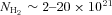 cm−2, we find cloud-averaged values X ∼ 2–4 × 1020 cm−2 K−1 km−1 s for solar-metallicity models.
1 INTRODUCTION
Carbon monoxide (CO), the second most abundant molecule in the interstellar medium (ISM), has now been observed for over 30 years to investigate the physical characteristics of the ISM. The lowest rotational levels are easily excited through collisions with molecular hydrogen (H2), by far the primary component of molecular gas in the ISM. Since H2 is difficult to detect directly, and the 12CO J=1−0 line occurs at a frequency (115.27 GHz) that is readily observable from the Earth, CO observations are well suited for probing the conditions of the molecular component of the ISM.
Accurately measuring the masses and velocities of gas within molecular clouds (MCs) is of primary importance for understanding star formation. CO observations of Galactic and extra-galactic MCs have provided a wealth of information about these properties, allowing for detailed modelling of the star formation process. However, uncertainty remains about exactly how to convert observed CO emission into fundamental physical properties of the dominant molecular component of the ISM.
The low rotational transition lines of CO are known to be optically thick, and therefore a considerable fraction of the emission from high-density regions must be self-absorbed. Nevertheless, a strong correlation is found between the CO intensity and the H2 column density  . A number of methods are employed to measure
  . These include mass determinations using observations of 13CO, which has lower optical depth than 12CO and so may be capable of tracing much of the MC gas (e.g. Dickman 1978). Alternatively, if MCs are in virial equilibrium, the 12CO linewidth may be used to estimate the virial mass (e.g. Larson 1981; Solomon et al. 1987). Independent mass measurements not involving CO include observations of γ-rays, which are produced when cosmic rays interact with the ISM. The molecular content is deduced when H i observations provide information about the amount of atomic material along the line of sight (Strong et al. 1988). Dust-based observations in the infrared may also provide indirect gas mass estimates, using appropriate dust-to-gas ratios (e.g. Dame, Hartmann & Thaddeus 2001; Pineda, Caselli & Goodman 2008; Leroy et al. 2009).
 is expressed as
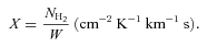
 (or gas mass) from CO observations.
A key assumption in using an X factor to derive gas masses is that the CO line is an approximately linear tracer of the bulk of the MC gas. Since the CO line is optically thick, however, it is not obvious why a linear relationship should hold. Extending the analysis of Dickman, Snell & Schloerb (1986), Solomon et al. (1987) advanced the ‘mist’ model in which an MC is composed of optically thick cloudlets that have well-separated velocities, such that the amount of self-absorption in the MC is small, and W is proportional to the total number of cloudlets along the line of sight, hereafter LoS. The assumptions implicit to this ‘mist’ model have not, however, been tested with radiative transfer modelling in realistic MC models.
Despite the correlations between W and  described above, there are in fact signs that no universal X factor is applicable to all sources. First, since the CO line is optically thick, observations of Galactic MCs show that beyond a threshold column density, W saturates so that the CO line no longer traces gas mass (Lombardi, Alves & Lada 2006; Pineda et al. 2008). Observations of low-metallicity systems such as the Small Magellanic Cloud (SMC) suggest X ≫ XGal (Israel et al. 1986; Israel 1997; Boselli et al. 1997; Boselli, Lequeux & Gavazzi 2002; Leroy et al. 2009, 2011). Theoretically, low-metallicity systems are expected to have lower CO abundances, which lead to lower CO intensities and thereby larger X factors (Maloney & Black 1988; Wolfire, Hollenbach & Tielens 1993; Israel 1997; Shetty et al. 2011, hereafter Paper I) provided that the other properties of the MCs (e.g. mass, size) do not vary greatly with metallicity (Glover & Mac Low 2011). Further, using independent dust-based measures of
  leads to X factor estimates that differ from X computed through the ‘virialized’ cloud assumption (Leroy et al. 2007, 2009; Bolatto et al. 2008). This discrepancy is taken as evidence that there are large reservoirs of molecular gas untraced by CO (Grenier, Casandjian & Terrier 2005; Planck Collaboration et al. 2011). One explanation for such a situation is that in the outer regions of MCs, CO cannot form efficiently due to poor self-shielding (Wolfire, Hollenbach & McKee 2010).
The discrepancies and range in the X factor estimates need to be understood in order to accurately interpret CO observations. One important issue related to the X factor is the dynamical state of MCs. Two well-known scaling relationships for MCs have been established in large part due to CO observations: the mass–size and linewidth–size relationships (Larson 1981), often referred to colloquially as ‘Larson’s Laws’. Assuming constant X, the MC masses M are found to be related to the projected size R through a power law with approximate index 2, M ∝ R2. Observed linewidths for MCs follow a power-law relationship with projected size σ∝ R1/2. Taken together, the interpretation of these relationships is that clouds are (approximately) in virial equilibrium, or ‘virialized’, so σ2≈ GM/R (Larson 1981; Dickman et al. 1986; Solomon et al. 1987; Myers & Goodman 1988). Alternatively, if MCs are virialized such that  , then X ∼σ2/(μGRW). If σ2/R and W vary little over the population of MCs, then X would have a uniform value.
An open question is whether the ‘mist’ model is applicable to turbulent media, as turbulence is now considered a dominant factor controlling the dynamics of MCs (e.g. Mac Low & Klessen 2004; McKee & Ostriker 2007, and references therein). In the first publication in this series (Paper I), we investigated how well CO can trace the underlying molecular gas using radiative transfer calculations on magnetohydrodynamic (MHD) models of MCs, which include a treatment of chemistry. We focused on velocity-integrated CO intensity, and compared probability distribution functions (PDFs) of W,  and CO column density NCO. We also assessed the X factor, again only considering velocity-integrated intensities. We showed that even though X may vary between different LoSs through a given MC, the cloud-averaged intensity produces X ≈ XGal within a factor of 3, from various models with different metallicities Z/Z⊙ = 0.3–1 and densities n0 = 100–300 cm−3. In this work, we focus primarily on the Milky Way MC model from Paper I, and investigate the properties that affect the derived X factor. Using radiative transfer calculations of turbulent chemo-MHD models, we perform a rigorous theoretical investigation of the qualitative models proposed to explain the observed X factor. We directly modify the cloud characteristics, such as temperature, density and velocity, and recompute the X factor to understand its dependence on those parameters. Two of our goals are to understand why the X factor is roughly constant for a range of systems, including Milky Way field GMCs, and to assess whether the ‘mist’ model is applicable to turbulent MCs.
This paper is organized as follows. In the next section, we provide an overview of the estimated X factor in various environments. We also discuss the results from Paper I in the context of observationally derived values. In Section 3 we review our method of modelling CO emission from turbulent MCs, and discuss some properties of the main Milky Way MC model. In Section 4, after discussing how the X factor is measured, we compare how X depends on the dynamic, chemical and thermal structure of the model MC. We investigate in detail the dependence of X on various cloud characteristics, such as temperature, H2 and CO densities, as well as the velocities. In Section 5, we compare our results to previous observational and theoretical efforts, and offer a new explanation for observed trends. Section 6 summarizes our interpretation of the observed X ≈ XGal and our conclusions regarding the parameter dependences of X.
2 OVERVIEW OF THE X FACTOR
As alluded to in the previous section, the X factor is found to be nearly constant when considering a specific class of sources, such as Galactic MCs, or a different value for ULIRGs. Yet, the analysis of the full spectrum of molecular environments generally portray a trend of decreasing X factor with increasing molecular surface density. Fig. 1 shows a compilation of observationally inferred X factors from various systems (Tacconi et al. 2008).
Compilation of estimated X factors from a range of systems, shown as a function of surface density. Figure reproduced from Tacconi et al. (2008), by permission of the AAS.
In Paper I, we analysed the X factor in various models with different metallicities Z/Z⊙ = 0.1–1 and densities n0 = 100–1000 cm−3. Fig. 2 shows the relation between the X factor and surface density Σgas or  from the models discussed in Paper I.2 The points show the mean X factor averaged in bins of Σgas, and the large points show the cloud-averaged X factor. At intermediate surface densities Σgas∼ 50–200 M⊙ pc−2, the cloud-averaged X factors for all but the very low Z = 0.1 model are ∼2–5 × 1020 cm−2 K−1 km−1 s ≈ XGal.
Mean X factor in bins of gas surface density Σgas (bottom axis) or  (top axis) for five models. The X factor is averaged in different Σgas bins. The value of
  is plotted on the midpoint value of Σgas of each bin. Each model is identified by different colours and symbols (and labelled in the legend). The large symbols show the global (emission-weighted) mean X factor and mean Σgas from each model.
Both Figs 1 and 2 show that X is larger than XGal in low-metallicity systems. As explained in Paper I, large X factor values at low metallicities and densities are primarily due to the low W, the integrated CO intensity, relative to  (equation 1). Systems with lower abundances of CO will of course have lower W. The formation of CO is highly dependent on the MC density, metallicity and strength of the background UV radiation field (see also Maloney & Black 1988; van Dishoeck & Black 1988; Glover et al. 2010; Glover & Mac Low 2011). However, H2 formation is not as sensitive to these properties, due to its ability to effectively self-shield. Thus, the relative abundance of CO compared to H2 can vary significantly within an MC, leading to a wide range in the X factor, even though the (emission-weighted) average of many different clouds may all result in a value ∼XGal.
Note that the low surface density regimes in Figs 1 and 2 are not directly comparable. The low surface densities in our numerical models correspond to diffuse regions in MCs with size ∼10 pc. In Fig. 1, the low surface density cases correspond to observations with low beam filling factors. These regions can have sizes ∼ kpc (or larger). Therefore, the objects in the two figures may differ in size.
At large surface densities (Σgas≳ 200 M⊙ pc−2), our turbulent models show an increase in the X factor, whereas the observations suggest a decreasing X factor. The increase of X with increasing surface density in our models occurs because in this regime the CO line is saturated, so that W remains constant even as  increases.
Our models only account for the effects of MHD, thermodynamics and chemical evolution. The sources at high surface densities in Fig. 1 are either the Milky Way centre or galaxies undergoing intense star formation activity (LIRGs and ULIRGs). The heating associated with star formation, as well as the large-scale rotation and turbulence of the ISM in these galaxies, is not captured by our models. These processes likely contribute to setting the X factor in such environments, and may be responsible for the observed trends in Fig. 1 at high Σgas.
In our current investigation of the X factor, we aim to understand which MC properties are responsible for X ∼ XGal in the 50–200 M⊙ pc−2 range. To carry out our analysis, we perform simple experiments by manually changing a number of physical parameters of our models. We then recompute the X factor, and assess which of the modified parameters most affect the resulting value of X.
2.1 Definition of the X factor

3 MODELLING METHOD
3.1 Numerical magnetohydrodynamics, chemistry and radiative transfer
To investigate how MC characteristics affect the X factor, we analyse MHD models of MCs that include a time-dependent treatment of chemistry. We perform radiative transfer calculations on these numerical models in order to solve for the CO level populations and compute the emergent CO intensity. The ratio of the H2 column density to the emergent CO intensity then gives the X factor (equation 1).
The MHD grid-based models follow the evolution of an initially fully atomic medium with constant density in a (20 pc)3 periodic box. Thermodynamics are coupled with chemistry to follow the formation and destruction of 32 chemical species, including H2 and CO, through 218 chemical reactions. Emission from CO and C+ are the primary cooling mechanisms in the dense and diffuse regions, respectively. Additionally, a constant background UV radiation field is included, which can photodissociate molecules in regions with insufficient shielding. The photoelectric effect is responsible for most of the heating in the diffuse regions, and in more dense regions heating is primarily due to cosmic ray interactions. Turbulence is driven on large scales (with wavenumbers 1 ≤ k ≤ 2) to maintain an approximately constant root mean square (3D) velocity vrms.
For a thorough description of the modelling method, we refer the reader to Glover & Mac Low (2007a,b) and Glover et al. (2010). In this work, we primarily consider the fiducial model chosen to match typical Milky Way MC conditions, which has an initial hydrogen nuclei density n0 = 300 cm−3, a metallicity Z/Z⊙ = 1, a background UV radiation field3 2.7 × 10⁻³ erg cm−2 s−1 and a time-averaged turbulent velocity vrms = 5 km s−1. The magnetic field is initially oriented along the  -axis, with magnitude 1.95 μG.
We use the radiative transfer code radmc-3d4 to calculate the emergent CO intensity. The level populations in each zone are calculated through the Sobolev approximation (Sobolev 1957), which uses velocity gradients across the faces of each grid zone to estimate photon escape probabilities. We employ the Einstein and collisional rate coefficients estimated by Yang et al. (2010) and provided in the LAMDA data base (Schöier et al. 2005). A full description of the radiative transfer calculation is provided in Paper I.
The radiative transfer calculations provide the CO intensities at each LoS position (x,y) at a given frequency ν (or velocity) bin, Iν(x, y). Besides the viewing geometry and the spectral resolution of the synthetic observation, the only other user-defined parameter required to perform the calculation is the microturbulent velocity vMTRB (see equations 2– 7 in Paper I). For our fiducial model, we use vMTRB = 0.5 km s−1. In the Appendix, we demonstrate that W or X does not strongly depend on this choice, for vMTRB∈ 0.25–0.75 km s−1.
Since we are interested in emission from all the gas in the simulation volume, the spectral channels span the full range in gas velocities. The position–position–velocity (PPV) cube provided by the radiative transfer calculations has a spatial resolution of 0.08 or 0.16 pc, corresponding to the extent of the zones in the 2563 or 1283 simulations, respectively, and a spectral resolution of 0.06 km s−1.
3.2 The fiducial Milky Way GMC model
Fig. 3 shows  and W of the fiducial Milky Way model MC, n300. Though the overall morphology of
  is evident in the CO image, there are some stark differences. Most notably, the brightest regions in the CO map (near the bottom) do not correspond to the region with the highest column density (near the top right). This discrepancy arises due to the high optical depth in the CO line. The differences between the observed emission and the underlying gaseous properties of these and other models are described in more detail in Paper I.
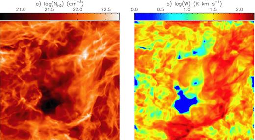
(a) Column density  and (b) integrated CO intensity of the Milky Way model MC.
Table 1 lists the mass and volume-weighted H2 number densities, temperatures and LoS rms velocities5〈v2los〉1/2=σv, los, along with the initial density n0 and box size L of model n300. Mass and volume-weighted quantities are defined as 〈f〉mass=∑fρdV/∑ρdV and 〈f〉vol=∑fdV/∑dV, respectively.6 The last row of Table 1 shows a reference value of the X factor:  .
.
Characteristics of standard ‘Milky Way GMC’ model (n300).
| Property | Value |
| Box size L | 20.0 pc |
| Initial atomic density n0 | 300.0 cm−3 |
 | 1098.0 cm−3 |
 | 145.9 cm−3 |
| 〈T〉mass | 19.8 K |
| 〈T〉vol | 51.7 K |
 | 2.4 km s−1 |
 | 2.4 km s−1 |
| 〈X〉ref | 1.9 × 1020 cm−2 K−1 km−1 s |
| Property | Value |
| Box size L | 20.0 pc |
| Initial atomic density n0 | 300.0 cm−3 |
| 1098.0 cm−3 |
| 145.9 cm−3 |
| 〈T〉mass | 19.8 K |
| 〈T〉vol | 51.7 K |
| 2.4 km s−1 |
| 2.4 km s−1 |
| 〈X〉ref | 1.9 × 1020 cm−2 K−1 km−1 s |
Characteristics of standard ‘Milky Way GMC’ model (n300).
| Property | Value |
| Box size L | 20.0 pc |
| Initial atomic density n0 | 300.0 cm−3 |
| 1098.0 cm−3 |
| 145.9 cm−3 |
| 〈T〉mass | 19.8 K |
| 〈T〉vol | 51.7 K |
| 2.4 km s−1 |
| 2.4 km s−1 |
| 〈X〉ref | 1.9 × 1020 cm−2 K−1 km−1 s |
| Property | Value |
| Box size L | 20.0 pc |
| Initial atomic density n0 | 300.0 cm−3 |
| 1098.0 cm−3 |
| 145.9 cm−3 |
| 〈T〉mass | 19.8 K |
| 〈T〉vol | 51.7 K |
| 2.4 km s−1 |
| 2.4 km s−1 |
| 〈X〉ref | 1.9 × 1020 cm−2 K−1 km−1 s |
As discussed in Paper I and Glover et al. (2010), the internal properties of the fiducial Milky Way cloud model take on a range on values. For example, the CO abundance relative to H2, fCO, can vary from ∼10−9 to 10−4. Similarly, the temperature, density and velocity also take on a wide range of values. Throughout our analysis, besides considering CO emission from the original model, we also consider models for which some relevant physical characteristics are modified, such as those with constant temperature or CO abundances. In this manner, we can quantitatively assess the effect of the various physical characteristics on the emergent CO intensity, and ultimately on the X factor.
4 RESULTS
4.1 Measuring the X factor
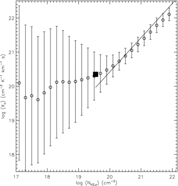
We begin by calculating the X factor through its traditional definition given by equation (1). Fig. 4 shows the mean X factor in bins of  as a function of
  from all LoSs through the fiducial model.7 As explained in Paper I, at the highest densities W does not increase with increasing
  due to the saturation of the CO line, resulting in X ∝
  . Nevertheless, the mean X factor only varies between (1.5 and 4) × 1020 cm−2 K−1 km−1 s for log
  = 21–22.5. Given this limited range and the extent of the error bars, a constant value at its emission-weighted mean value8 (shown by the large filled circle in Fig. 4) adequately describes the X factor for this model. This mean X factor value 〈X〉 = 2.2× 10²⁰ is in good agreement with the reference value provided in Table 1, 〈X〉ref = 1.9 × 10²⁰. We now consider the terms
  and W in detail, and their relationship to the physical properties of the model.
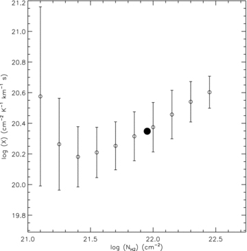
X factor from the Milky Way model MC. The open circles and error bars indicate the mean and standard deviation of the X factor in bins of  . The solid circle shows emission-weighted mean X factor of the whole model (〈X〉 = 2.2 × 1020 cm−2 K−1 km−1 s) at the mean column density (
 cm−2, corresponding to
  202 M⊙ pc−2).
 is computed along the same LoS and in velocity bins that match the spectral channels of the CO observation, then a column density cube of
  can be constructed which has the same configuration as the observed CO PPV cube.
 , intensity TB and adopted channel width Δv (in our case, 0.06 km s−1):
Fig. 5 shows how this ‘3D X factor’ depends on the column density for the Milky Way model cloud. Here,  extends to much lower values than the values of
  shown in Fig. 4, since the volume densities are integrated over a more limited region (in velocity space).
Xν versus  from the Milky Way model MC. The mean and standard deviation of Xν in bins of
  are shown as circles with error bars. The solid square shows emission-weighted mean Xν of the whole model (〈Xν〉 = 2.2 × 1020 cm−2 K−1 km−1 s) at the mean column density (
 cm−2). Line shows
  at
at  .
.
The emission-weighted mean ‘3D X factor’ is equal to X factor computed in its usual way, shown in Fig. 4. However, at high densities, Xν is significantly larger than X, reaching values ≳1022 cm−2 K−1 km−1 s, whereas the 2D X factor is always ≲1021 cm−2 K−1 km−1 s. From Fig. 5, it is clear that the CO line is saturated at column densities (per frequency bin) above the mean column density  cm−2, as indicated by the
  line, where
  is the mean brightness temperature in PPV regions where
 .
.
The discrepancy at high column densities between X and Xν is due entirely to the differences between W and TBΔv. On a given LoS, W is the summation of TBΔv through all velocities in the PPV cube. Fig. 6 shows these quantities as a function of  or
or  , respectively. Clearly, W continues to increase beyond
  ≳ 1021 cm−2, whereas TBΔv is saturated. Since Δv is constant, this means that TB saturates at a value ∼13 K.9
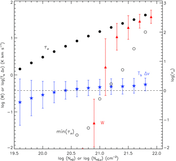
Intensity (left ordinate) and optical depth (right ordinate) plotted against column densities. Triangles show the mean-integrated CO intensity W as a function of total column density  (2D). Stars show the analogous relationship from (3D) PPV cubes, TBΔv versus
  . Filled circles show the mean optical depth τν, and the open circles show the minimum value of τν in the
  bins. Dashed line corresponds to τν = 1.
The mean and minimum value of τν, in bins of  , are also shown in Fig. 6, with the scale given on the right ordinate. Though TBΔv does not vary much in the range of the high column densities shown in Fig. 6, a trend of increasing TBΔv with column density is apparent until the
  cm−2. At column densities
  cm−2, all values of τν > 1, indicating a complete saturation of TBΔv.
The fact that velocity-integrated brightness temperature W still increases beyond  cm−2, where the line is saturated, indicates that numerous optically thick regions at different v contribute to W. This results in the saturation of the integrated intensities occurring at higher column densities than the saturation of the intensities in the PPV cube, as evident at the highest
  in Fig. 6.
A consequence of the line saturation described above is that the amount of gas that is untraced depends not only on the density, but also on the velocity. For instance, a ‘cloudlet’ or parcel of dense gas with similar velocity as another parcel along a LoS, but separated in space, would not contribute extra flux to TB, or the W map. On the other hand, a ‘cloudlet’ with much different velocity along the LoS would be traced, detected as higher TB at a different location in the velocity axis of the spectrum, and thus contribute to the integrated intensity W. Consequently, LoSs with (dense) gas spanning a larger range in velocities will have larger Ws. This concept of optically thick dense ‘cloudlets’ is the basis of the ‘mist’ model put forth by Solomon et al. (1987) to explain the uniformity in the X factor in Galactic GMCs. We return to the applicability of the ‘mist’ model in Section 4.5.
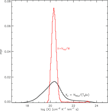
The differences in the relationships between W and TBΔv with column density (Fig. 6) lead to the variations between X and Xν (Figs 4 and 5). The (2D) X and (3D) Xν distributions are shown in Fig. 7. Though the peak value of the two distributions is similar, there is a much larger distribution in Xν. In considering synthetic observations with different spectral resolution, we find that the range in Xν depends on Δv, but that 〈Xν〉 = 2.2 × 1020 cm−2 K−1 km−1 s consistently. As discussed, there are lower column densities  in a PPV cube compared to
  . For such densities, the line is often optically thin, and there is a range of possible emergent intensities for a given column density (Fig. 6). This results in a larger range in Xν compared to X.
Taken together, the limited range in the 2D X factor shown in Figs 4 and 7 only occurs when the CO intensities are integrated over all velocities, and densities over the whole LoS. Effectively, a limited range in the X factor only results when combining the detailed velocity, as well as density, structure along the LoS. This is indicative of the fact that the velocity range plays a crucial role in setting the X factor.
Of course, integrating the observed brightness temperatures over a limited range in velocity is not practical, as obtaining  is not readily feasible in observational data sets. Nevertheless, such an analysis has underscored that the X factor depends on the total velocity width of the cloud, as explicitly evident in equation (4). But, how does the detailed velocity structure, such as its relationship with the size of emitting regions, affect the X factor? Further, what is the relative contribution of ∫dv compared to the other terms
  and TB in equation (4)? To address these questions, we investigate in detail the role of each quantity in determining the nature of the CO emission, and their relationship to intrinsic cloud properties.
4.2 X factor dependence on temperature
Due to the thermodynamics in the chemical-MHD model, the gas has a range of temperatures. As indicated in Table 1, the model MC has a (volume-weighted) mean T ≈ 50 K, with a dispersion σ≈ 44 K. This range in temperatures will also result in a range in the X factor, since the observed brightness temperature depends on the gas kinetic temperature (equation 2).
To test the sensitivity of the X factor to the temperature distribution, we artificially set all temperatures in the model to a constant value, and then perform the radiative transfer calculations. The resulting maps are then compared with the original CO map. Any discrepancies can be attributed to the differences in temperatures.
This is illustrated in Fig. 8, where (a) shows the original distribution of X, and (b)–(d) show the X factors for constant temperatures of 20, 50 and 100 K. The histograms from the model with the original temperatures are provided in each panel as dashed lines.
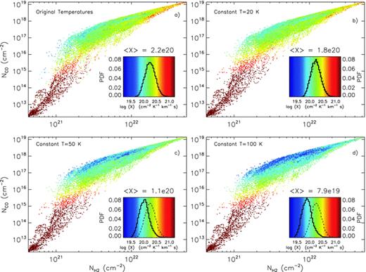
The variation of the X factor with gas temperature. The position of each point shows the relationship between  and NCO. The colour of each point identifies the value of the X factor, computed through equation (1), with the colour scale and distribution given in the inset plots. The emission-weighted mean value 〈X〉 is indicated in each plot. (a) Original model n300, (b) model n300, but with constant T = 20 K, (c) constant T = 50 K and (d) constant T = 100. In (b), (c) and (d), X factor distribution from original simulation in (a) is shown as thin dashed histogram.
The constant temperature T = 20 K model, equal to the mass-weighted temperature (see Table 1), provides an X factor distribution that is very similar to the original model (Fig 8b). This is expected since most of the CO is located in dense regions where T ≲ 20 K. The relationship between X,  and NCO is also rather comparable to the original relationship. Note that for both the original and constant T = 20 K models, the highest and lowest values of
  have large X (cf. Fig. 4). The differences between the 20 and 50 K model suggest that the X factor is more sensitive to the mass-weighted rather than the volume-weighted temperatures.
Fig. 9 shows the mean X in bins of  from the original model (as in Fig. 4), along with two reference values obtained directly from the simulation. The red stars show X computed using the mass-weighted LoS velocity and global mass-weighted temperature. The blue triangles show the corresponding X from the volume-weighted quantities. Along LoSs with column densities lower than ≲1021.8 cm−2, the CO fraction decreases, thereby decreasing W (see Paper I and Section 4.3.2). Thus, the simple relationships between X, T and vlos cannot reproduce the X factor at low column densities. At column densities ≳1021.8 cm−2, however, the X factor computed using the mass-weighted temperature agrees fairly well with the original X factor. The X factor computed from the volume-weighted temperature systematically underestimates the X factor. These trends indicate that the densest regions contribute most to setting W, and thereby the X factor.
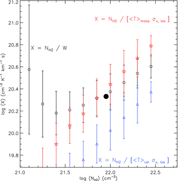
X factor (black circles) from the Milky Way model MC, as in Fig. 4. The emission-weighted mean X at the mean column density is shown by the large solid circle. Red stars show the X factor computed by  , and blue triangles show
  . 〈T〉mass and 〈T〉vol are the global mass- and volume-weighted temperatures, given in Table 1. σv, los is the mass-weighted rms velocity (which is equal to the volume-weighted rms velocity) along each LoS.
As indicated in Fig. 8, clouds with higher temperatures produce lower X factors, as would be expected from equations (1)–(2). From 〈X〉 = 1.8 × 10²⁰, 1.1 × 10²⁰ and 7.9 ××1019 cm−2 K−1 km−1 s at T = 20, 50 and 100 K, respectively, we find an approximate scaling 〈X〉∝ T−0.5. The range in the X factors in the modified-temperature models is, however, similar to the original model. This indicates that the range in temperatures in model n300 is not responsible for the range in the X factor. As a result, it is either the range in densities or the velocities which produce the distribution in the X factor.
We note that an increase in temperature to 100 K is likely accompanied by other variations in the MC structure, such as a decrease in  and possibly fCO if the high temperature is due to a high star formation rate. As such, models for which the temperatures are manually scaled to high values are likely omitting real environmental effects that would affect the X–T relationship.
4.3 X factor dependence on density
We turn our attention to the X factor dependence on density. Any given cloud will have a range in volume and column densities, in both H2 and CO. If W depends linearly on  , then there would certainly be a constant X factor along all LoSs. However, as discussed in Paper I, W generally does not have a straightforward scaling with the column density NCO, especially at large NCO due to the high opacity of CO (see Section 4.1). Further, NCO does not directly trace
  . This lack of correlation between W and
  results in a distribution of X along different LoSs for a given MC. We focus on how the volume density and CO abundance affect the X factor.
4.3.1 X factor dependence on volume density
To test whether the X factor is more sensitive to  or to
or to  , we consider a model with a higher volume density than model n300. This model (n1000) only differs from model n300 in its initial atomic density of 1000 cm−3. As described in Paper I, most of the carbon in this model is incorporated into CO, and so there is a very good correlation between NCO and
  (see fig. 5c in Paper I).
As explained in Paper I, for this high-density model the effect of line saturation is clearly apparent in the X factor computed through equation (1). Fig. 10 shows the relationship between X and  for model n1000. The line is not a fit, but rather the relationship
  , where
  70 K km s−1 is the mean-integrated intensity from this model. We see that X invariably increases with
  , as would be expected if the line were saturated.
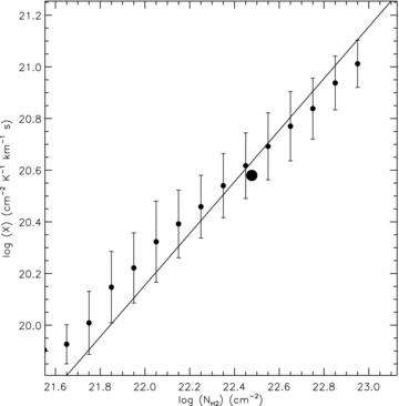
X factor versus  from model n1000, which has box size (20 pc)3. The line shows
  , with
  = 70 K km s−1. The large circle shows 〈X〉 = 3.8 × 1020 cm−2 K−1 km−1 s at
 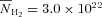 cm−2, or
  672 M⊙ pc−2.
The X– relationship for model n300 (Fig. 4) is quite different from the relationship from model n1000, due partly to the larger maximum column density in model n1000 and lower minimum column density in model n300. We investigate whether the total column density, which occurs explicitly in equation (1), is responsible for the increase in X at large
  in model n1000. We perform the radiative transfer calculations on a model which is similar to n1000, but whose box length is decreased by a factor of ∼3 to 6 pc. In this n1000-L6 model, the lower column densities allow the background UV radiation to penetrate further into the cloud, leading to more CO photodissociation. Nevertheless, this model should have similar H2 column densities to the n300 model, since H2 can self-shield more efficiently. On the other hand, the volume densities in n1000-L6 will be very similar to those in the n1000 model.
Fig. 11 shows the X– relation for this n1000-L6 model. The line shows
  , with
  K km s−1 for this model. Here, 〈X〉 is similar to the n300 model. The X–
 relation is not as well reproduced by the
  line as model n1000 in Fig. 10. Nevertheless, the X factor clearly increases with
  . Compared to model n300 (Fig. 4), X is similar for
  ∼1022–1022.5 cm−2, but there are significant differences at lower
  , especially ≲1021.5. Thus, the X factor, even when calculated using the total column density(equation 1), depends on the volume density
 , rather than just the column density
 . Note, however, that when averaged over all lines of sight, 〈X〉 decreases by only 15 per cent even though n0 increases by a factor of 3.3.
X factor versus  from model n1000-L6, which has initial density 1000 cm−3 and box size (6 pc)3. Line shows
  , with
  = 49 K km s−1. The large circle shows 〈X〉 = 1.9 × 1020 cm−2 K−1 km−1 s at
 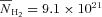 cm−2 corresponding to
  204 M⊙ pc−2.
4.3.2 X factor dependence on CO abundance
Besides containing a range in densities, there is also a range in CO abundances at a given H2 density, as is evident in the column density relationships in Fig. 8 (see also Paper I and Glover et al. 2010). In order to investigate how this distribution contributes to the X factor, we reset the CO abundance with a constant fCO= nCO/ ratio, and then perform the radiative transfer calculations.
Fig. 12 shows the X factor– relation for (a) the original model, as well as those with (b) constant fCO = 10−4, (c) 10−5 and (d) 10−6. Also shown in each panel is the line corresponding to the
  relation, indicating complete saturation of the CO line.
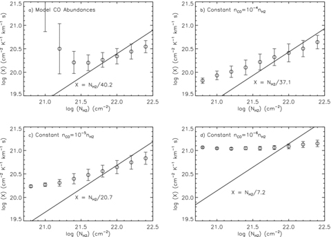
The X factor– relationship from model n300, as in Fig. 4(a), but with the CO number density reset to be (b) 10−4, (c) 10−5 and (d) 10−6× nH2. Line in each plot shows
  relation.
With the original abundances, the  relationship is close to the model values only at the highest column densities. At densities ≲3 × 1021 cm−2, the overplotted line underestimates X. In this regime, CO emission is not saturated. Fig. 12(b) is analogous to the limiting scenario where all the atomic carbon and oxygen is converted to CO, so that fCO = 10−4. For this model, the
  relation is similar to the data above
  cm−2, indicating that the CO line is nearly fully saturated. In Figs 12(c)–(d), with lower fCO, line saturation becomes less and less important, especially at lower column densities, finally resulting in a constant X and
  relation for fCO = 10−6.
In general, the CO line becomes saturated in regions with the highest CO abundance. With constant fCO = 10−4, X increases with increasing  everywhere, and the CO line is completely saturated at column densities ≳1021.5 cm−2 (Fig. 12b), resulting in
  . At lower CO abundances, W increases with increasing column density. This results in a shallower slope in the X–
 relation. At very low fCO = 10−6, W is directly proportional to
  , so that X is constant at all
  . Taken together, clouds with both low and high CO abundances will tend to have a more limited range in X than a cloud with only large fCO, which would have X ∝
  .
.
Notice that in Fig. 12(d), X = 1021 cm−2 K−1 km−1 s for the model with CO abundance fCO = 10−6. This is the quoted abundance in diffuse Milky Way gas observed by Burgh, France & McCandliss (2007) and Liszt et al. (2010). However, Liszt et al. (2010) find X ≈ 3 × 10²⁰≈ XGal, which is a factor of ∼5 lower than the resulting value in Fig. 12(d). The discrepancy is likely due to the combination of the differences in temperature and linewidths between the ‘diffuse’ MCs and more massive giant MCs. The diffuse ISM has a higher temperature, up to ∼100 K. As we demonstrate in Section 4.2, such high temperatures may account for a significant fraction of the difference. Further, observations of low column density LoSs probably trace a larger volume of the Galaxy, thereby including gas with a wider range in velocities than those found in MCs. As we discuss in the next section, larger velocities may lead to lower X factor values. Nevertheless, note that the discrepancy may be partly due to the fact that in this numerical experiment, we artificially fix the CO abundance. The metallicity and self-shielding are not self-consistently tracked in these experiments.
4.4 X factor dependence on velocity
In order to test the sensitivity of the X factor to the velocity vlos or the integral over dv appearing in equation (4), we consider MC models with different velocity fields. In the MHD simulations, turbulence is generated by continuously driving the gas velocities with uniform power between wavenumbers 1 ≤ k ≤ 2. In the standard Milky Way MC model presented so far, the saturation amplitude of the 1D velocity dispersion is 2.4 km s−1.
We test the effect of velocities by performing experiments on two different sets of models for which the velocities differ from the fiducial n300 model. The first set of models have different driven turbulent velocities. In these experiments, the other parameters of the simulations are identical to that from model n300 – only the saturated-state (3D rms) velocities differ by factors of 0.2 and 2. The second set of models are simply the original n300 models, but for which the velocities in each zone are manually modified. As discussed in Paper I, the chemical evolution is not strongly affected by the velocity field. It is the metallicity, density and background UV radiation field which are the primary factors determining CO formation (see also Glover et al. 2010; Glover & Mac Low 2011). Given the insensitivity of molecule formation to the velocity field, we can directly modify the velocities in model n300. We thus consider models with chosen velocity dispersions, where all the other parameters are equivalent to those in model n300.
4.4.1 Different levels of turbulence
Fig. 13 shows the linewidth–size relations for clumps in the MHD models. ‘Clumps’ are identified directly from the simulation (in the 3D density cube), through dendrograms (Rosolowsky et al. 2008). The dendrogram10 algorithm identifies contiguous structures through iso-density contours. The linewidth of each clump is computed from the dispersion in the corresponding region from the 3D vz-cube.11 As evident in Fig. 13, the linewidth–size relationship can be reasonably expressed as a power law σ∝ Ra. For the original n300 model (black circles) the best-fitting exponent a = 0.45. This is in good agreement with the observed linewidth–size relationship (e.g. Larson 1981; Solomon et al. 1987; Heyer et al. 2009). At small radii approaching the resolution limit of the simulation, the velocities approach a minimum threshold corresponding to the microturbulent velocity of 0.5 km s−1. This chosen value of the microturbulent velocity is greater than the thermal velocity due to the observed linewidths at ∼0.1 pc scales. At large scales, the 1D linewidths ∼2.4 km s−1 are the overall dispersion in the LoS velocities.
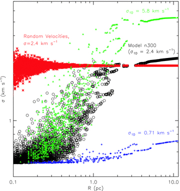
The linewidth–size relationship from model n300. Structures are identified directly from the 3D simulation. The linewidths σ are computed by taking the dispersion of the (1D, or vz) velocities from the identified structures in the simulations (black, blue and green) or from a Gaussian distribution with a dispersion of 2.4 km s−1 (red).
The blue and green points in Fig. 13 show the σ− R relationship from simulations with different forcing amplitudes, with 3D vrms≈ 1 and 10 km s−1, producing LoS velocity dispersions of 0.71 and 5.8 km s−1, respectively.12 For these simulations, the best-fitting power laws produce a = 0.08 and 0.61, respectively. The red points in Fig. 13 show the linewidth–size relationship from a model similar to n300, but with the velocities drawn from a random distribution with σ = 2.4 km s−1 (which produces a = 0).
Fig. 14 shows the relationship between X,  and NCO from the original n300 model, along with the models with different velocity fields. In Figs 14(b)–(f), the velocities vary due to a different turbulent forcing amplitude, or simply due to replacing the velocities from the n300 MHD simulation with a Gaussian distribution. As discussed, the original velocities in model n300 (Fig. 14a) have an LoS dispersion of σ = 2.4 km s−1, due to turbulent forcing with 3D (rms) mean dispersion vrms = 5 km s−1.
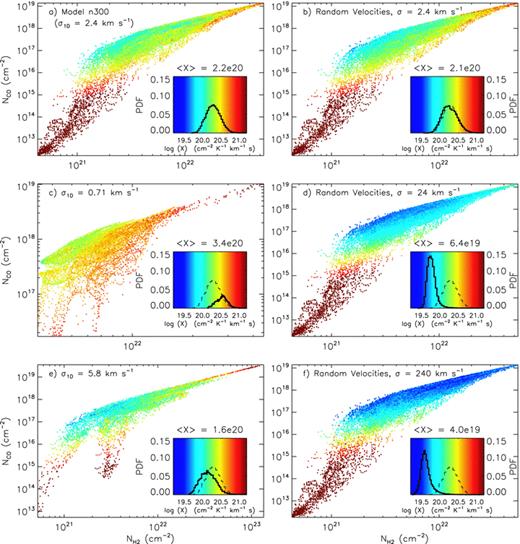
The variation of the X factor with  and NCO, as in Fig. 8, but for models with different internal velocity fields. (a) Original model n300, which has σ1D = 2.4 km s−1, (b) model n300, but with velocities replaced from a Gaussian distribution with σ = 2.4 km s−1, (c) model with σ1D = 0.71 km s−1 (vrms = 1 km s−1), (d) n300, but with Gaussian velocities with σ = 24 km s−1, (e) model with σ1D = 5.8 km s−1 (vrms = 10 km s−1) and (f) n300, but with Gaussian velocities with σ = 240 km s−1. In (b)–(e), the X factor distribution from the fiducial n300 model in (a) is shown as the thin dashed histogram. The emission-weighted X factor 〈X〉 is indicated in each panel.
Figs 14(c) and (e) show the X factor from models where the turbulent forcing is varied from the original n300 to yield σ1D≈ 0.71 km s−1, or σ1D≈ 5.8 km s−1, respectively. Fig. 13 demonstrates that the velocities of the large-scale structures in these model vary by a factor of ∼3 above and below the original n300 model, but are rather similar on the smallest scales due to the imposed microturbulence. Because the turbulent driving varies, the gas in these models contain different amounts of CO, and different temperatures. Comparing the other properties of these models (in Table 1), the lower velocities in the 0.71 km s−1 model result in lower temperatures (〈T〉vol = 24 K), and lower amounts of total CO (as well as H2,  cm−3). The 5.8 km s−1 model, on the other hand, has 〈T〉mass = 27 K. Nevertheless, the X factor for these models is both within ∼50 per cent of the n300 value (〈X〉 = 3.4 × 10²⁰, 2.2 × 10²⁰ and 1.6 × 1020 cm−2 K−1 km−1 s, respectively, for σ1D = 0.71 km s−1, 2.4 km s−1 and 5.8 km s−1).
4.4.2 Purely Gaussian velocities
The panels on the right-hand side in Fig. 14 show the X factor from model n300, but with the velocities replaced with random values drawn from a Gaussian distribution with σ = b) 2.4, d) 24, and e) 240 km s−1. For the σ = 2.4 km s−1 model, the linewidth–size relationship differs significantly (Fig. 13) from the fiducial model n300. The dispersions are similar on large scales, by design. However, at smaller scales the dispersions in the original model decreases, whereas there is a constant dispersion on all scales in the modified model. Nevertheless, the X factor distribution is very similar to the original model n300. The globally averaged X factor from the original model is recovered. That the X factor is very similar to the original model suggests that the details of the velocity structure, and its relationship to other physical properties such as mass or size, do not play an important role in determining the X factor. In particular, clouds with very different linewidth–size relationships from σ∝ R1/2 may produce X ≈ XGal.
In models with random velocities having 1D dispersions σ = 24 and 240 km s−1, the X factor is systematically lowered, to 〈X〉 = 6.4 × 10¹⁹ and 4 × 1019 cm−2 K−1 km−1 s, respectively. Therefore, the integrated CO intensity W is not sensitive to the velocity structure, but only the extent of the range in velocities. This occurs because with larger velocity differences between regions along a LoS, more CO line photons are able to escape the cloud and ultimately be detected, resulting in an increase in W. Increasing Δv thereby effectively reduces the percentage of mass that has τ > 1 (and is therefore ‘invisible’), so that more CO becomes visible. Notice that the difference in the X factors of the models with dispersions of 24 and 240 km s−1 (Figs 14d and f) is modest. Thus, X does not simply scale inversely with σ. In fact, the results from models with σ = 2.4, 5.8 and 24 km s−1 show a behaviour closer to X ∝σ−1/2 than X ∝σ−1. We return to this point in Section 4.6.
Of course, the range in velocities must be sufficiently well-sampled, so that there are no significant velocity gaps, which will indeed be the case in MCs. The σ = 24 and 240 km s−1 models have a large range in velocities, and consequently, likely have under-resolved velocity gradients. In the Appendix, we discuss how radiative transfer calculations may provide inaccurate intensities in regions where the velocity gradients are poorly resolved, and how our analysis accounts for this effect.
4.5 Does ‘cloud counting’ result in a constant X factor?
One explanation for the lack of variation in the X factor in the Galaxy is that the integrated CO intensity is a measure of the number of optically thick ‘cloudlets’ along the LoS. This is known as the ‘mist’ model proposed by Solomon et al. (1987). Since we have knowledge of all the relevant quantities affecting the X factor, we can test this idea by inspecting the characteristics of the gas contributing to the observed emission.
Fig. 15 shows the spectrum from two LoSs. The top panels show TB and τ at each spectral channel. The bottom panels show the corresponding volume density and velocity. For reference, the observer is situated beyond LoS position 0 in panels c–d, so that observed line photons are travelling from high LoS position towards lower LoS position (to the left on the plots).
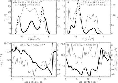
Top panels – CO spectra (lines – left axis) and optical depth (circles – right axis), and bottom panels – H2 volume densities (thin – left axis) and LoS velocities (thick – right axis) from two LoSs in the n300 simulation. The corresponding integrated intensities and X factors are listed in (a)–(b), and the column densities are listed in (c)–(d).
Both LoSs A and B have similar total column densities, 1.0 and 1.1 × 1020 cm−2, respectively. However, the integrated intensities differ by a factor of ∼2.5. Perhaps surprisingly, LoS A, which has slightly lower column density, has a much higher intensity. As a result of this difference in W, the resulting X factors for these LoSs as computed from equation (1) also differ.
The differences in the total intensities and line shapes from the LoSs depicted in Figs 15(a)–(b) can be understood by inspecting the density and LoS velocity distribution shown in Figs 15(c)–(d). LoS A has relatively low density gas ≲100 cm−3 in the majority of positions along the LoS, at position 0–17 pc. Near LoS position 17 pc, there is a sharp jump in density, and an associated perturbation in velocity. The lowest LoS velocities associated with this shock, ≲−5 km s−1, are unique to this particular region along the LoS – no other region along this LoS has similar velocities. Accordingly, observed emission in the −5 to −7 km s−1 range originates from this high-density, optically thick cloudlet. Emission at velocities −3 to 4 km s−1 from this cloudlet may be absorbed by the gas lying along the LoS with similar velocities. However, this gas has very low column density, and so in fact does not significantly attenuate the emission from the shock. Thus, the whole line profile in the −7 to 3.5 km s−1 range is due to the high-density shock. Only the weak remaining emission at velocities ≳4 km s−1 is due to gas at positions ≲3 pc. We discuss some numerical effects in regions of such high-velocity contrast in the Appendix.
The LoS in Fig. 15(b) does not have any gas with  > 2000 cm−3. There are numerous optically thick regions, with a significant overlap in velocities. Some regions, such as the peak near position 8 pc, have small velocity gradients, while others contain a large range in velocities, as the peak near position 14 pc. Due to the large overlap in velocities, especially at −4 km s−1, the integrated optical depth reaches very high values up to 170. The combination of velocity overlap and lower density gas results in LoS B having a lower integrated intensity than LoS A.
Fig. 16 shows two other LoSs with lower column densities; these have equivalent  cm−2. Yet, the integrated intensity varies by a factor of ∼3, resulting in an equivalent discrepancy in the X factor. Judging by the optical depth profile, there appears to be either one or two cloudlets. However, the detailed velocity and density profiles show that the structure is much more complex.
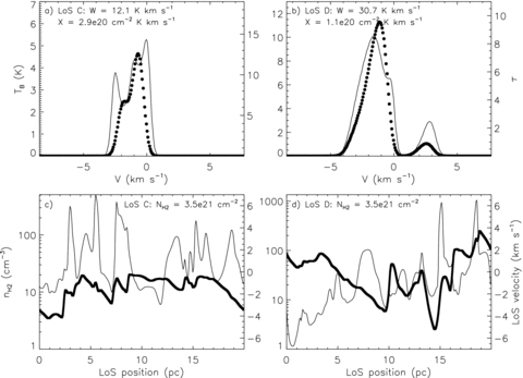
Almost all of the gas along LoS C has densities ≳10 cm−3. Most of the gas velocities, especially those associated with the density peaks with  cm−3, lie in the range −3 to −1 km s−1. There are many density peaks with overlapping velocities, but the resulting line profile has only three peaks. Since τ > 1, the observed intensity at a given velocity emerges from the last density peak along the LoS with the given velocity. Thus, much of the emission from LoS position >10 pc is absorbed. By rerunning the radiative transfer on this LoS by excluding some of the gas, we have verified that a significant number of CO line photons are absorbed. We provide examples demonstrating this scenario in Section 4.6.
For LoS D, a fraction of the gas has  cm−3. This LoS has two well-defined peaks in the line profile. These peaks are centred on −3 and 3 km s−1. At those velocities, there are two distinct cloudlets with
  cm−3. Clearly, the emission from LoS D comes from the most dense regions along the LoS. Since they are well separated in velocity, both are easily detected and contribute to a larger integrated intensity than LoS C.
The comparison of observed profiles, densities and velocities in Figs 15 and 16 suggests that the simple ‘mist’ model does not accurately capture the complexity intrinsic to line radiative transfer from a turbulent medium. In the comparison of LoS A and B in Fig. 15, both of which have a large  , A has one true cloudlet with very high density. This cloudlet is only present in a localized region along the LoS, but contains a large range in velocities, and therefore is the source of most of the observed emission. Other emitting regions with different velocities only contribute slightly to the spectrum, due to their significantly lower densities. LoS B has numerous lower density cloudlets, many of which have similar velocities. The integrated intensity is lower, though the total amount of gas along this LoS is slightly larger than LoS A.
In the comparison of low-density LoSs in Fig. 16, both LoSs have a few regions with clear density peaks. However, the dominant cloudlets in LoS D have larger density, and span a larger range of velocities. Thus, LoS D has a higher total intensity than LoS C even though the total column density in both LoSs is equivalent.
The ‘mist’ model would predict that LoSs with more high-density cloudlets would have higher integrated intensities, since the cloudlets are separated in velocity. However, the comparison of LoS A and B shows the opposite: one very dense cloudlet with a large velocity gradient may be responsible for the whole LoS profile. This integrated intensity W may be larger than that from a different LoS with a larger number of cloudlets, but nevertheless a similar total column density and total velocity width. Further, two LoSs with equivalent  and similar number of cloudlets may have different W if one LoS has overlapping cloudlets in velocity space, while the other LoS has well-distributed cloudlets in velocity space. This effect is partly at work in the comparison of LoS C and D in Fig. 16.
We have shown that in a turbulent medium, emitting cloudlets do in fact overlap in velocity space (see also Ballesteros-Paredes & Mac Low 2002; Shetty et al. 2010), and that individual cloudlets may have a range in velocities, thereby dominating the emission at all velocities in that LoS. These factors all compromise any simple relation between W and  , and therefore any direct scaling between X and
  . Of course, this analysis considers individual LoSs through an MC, whereas the idea of a constant X factor is usually discussed in the context of whole MCs. Accordingly, we next consider the cloud-averaged CO spectrum.
4.6 Cloud-averaged X factor and spectra
Fig. 17 shows the averaged spectrum for the whole n300 cloud model, as well as model n300 where the velocities are manually replaced with σ = 24 km s−1 (see Fig. 14d). Each point shows the mean brightness temperature of each channel in the synthetic observation. The integrated intensity of this spectrum is W = 40.2 and 137.5 K km s−1 for the fiducial and velocity-altered model, respectively.
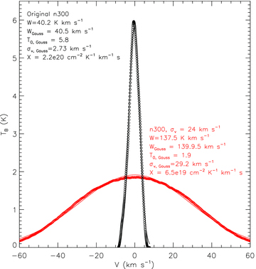
Averaged spectrum from model n300 (black), and model n300 for which the velocities were replaced from a random distribution with σ = 24 km s−1(red). Lines show best-fitting Gaussians. Integrated intensity, fit Gaussian parameters and X factor are listed for both models.
The best-fitting Gaussians to the averaged spectra are also shown in Fig. 17. The spectra are very well fit by Gaussians. Using the peak and dispersion of the Gaussian fit, the corresponding integrated intensities reproduce the true integrated intensities. Using W along with the mean column density  cm−2 in equation (1) results in X = 2.2 × 10²⁰ and 6.5 × 1019 cm−2 K−1 km−1 s for the original and 24 km s−1 models, respectively. These values of the X factor are equivalent to the emission-weighted mean X found in Section 4.1 and are listed in Fig. 14. The X factor value for n300 is nearly identical to the reference value in Table 1. For the altered velocity model, 〈v2z〉mass = 24 km s−1 so the reference
  cm−2 K−1 km−1 s. This value is significantly lower than X determined by the spectrum, largely due to the fact that TB/〈T〉mass is a factor of 3 lower for the 24 km s−1 model than for model n300 with σ1D = 2.4 km s−1. Therefore the mass-weighted quantities 〈T〉massand 〈v2z〉mass1/2cannot fully account for W. We note that the linewidths of the observed spectrum are slightly larger than the intrinsic velocity dispersion. This is due to some extent to our choice of the microturbulence, which we discuss in more detail in the Appendix.
The cloud-averaged spectra in Fig. 17 show very smooth profiles, and do not demonstrate any of the variability seen along individual LoSs. Clearly, the cloud with a larger velocity dispersion is brighter because the emission from more gas with a larger dispersion is able to escape the cloud. Even though both models have the same mass, their integrated emission differs by a factor of 3.4. This is due to a combination of a larger velocity dispersion (by a factor of ∼10), and a lower peak brightness temperature (by a factor of ∼3) for the 24 km s−1 model compared to model n300. As a result, the use of the integrated intensity alone, or any X factor, would provide inaccurate mass estimates.
We have demonstrated that there is no simple relationship between W and  in highly turbulent clouds (see also Paper I). This lack of correlation is due to the combination of the optically thick nature of CO, and the complexity in the structure of CO bright regions: emitting gas along individual LoSs sometimes overlaps in velocity space and sometimes does not, and even lower density gas not necessarily found in cloudlets contributes significantly to the observed intensity. Under such circumstances, there should be significant amounts of gas that is untraceable in the CO line.
Fig. 18 shows the averaged spectrum of three models. The black spectrum is from the original n300 model. The red and blue points show the results of the radiative transfer calculations from model n300, but only when gas with  cm−3 and >1000 cm−3 is included in the calculation, respectively. The CO and H2 density is set to zero in zones with
  cm−3 or >1000 cm−3, respectively.
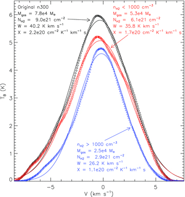
Averaged spectrum from original model n300 (black circles), along with spectrum from the original model but only gas with  cm−3 (red squares) and >1000 cm−3 (blue triangles), is considered. Lines show best-fitting Gaussians.
The gas mass in the model that has  cm−3 is 5.3 × 10⁴ M⊙, which is roughly two-thirds of the total mass in the original n300 model. However, the integrated intensity from this model is 90 per cent of that from model n300. The total mass at
  cm−3, 2.5 × 10⁴ M⊙, accounts for the remaining one-third of the mass in model n300. But the integrated intensity from this model is 26.2 K km s−1, which is 65 per cent of the total W of the original model.
Due to the significant amount of self-absorption occurring in both low- and high-density gas, removing some gas simply allows other gas along the LoS to become ‘visible’. There are LoSs where some CO emitting regions go completely undetected, since other optically thick gas lying in the same LoS with similar velocities will absorb its emission. Consequently, a spectrum from a given LoS may depend on the observing direction. For example, if the observer were located at LoS position >20 pc in Figs 15 and 16, instead of at LoS position <0 pc, the spectra may have different profile shapes. We have indeed found such discrepancies in many LoSs. This is further confirmation that there is no simple correlation between  and W. We stress again that the use of a constant X factor for numerous clouds will not provide reliable estimates of the molecular mass.
5 DISCUSSION
5.1 Why is the Galactic X factor found to be nearly constant?
After investigating the dependence of the X factor on the physical characteristics of synthetic MCs, we are now in a position to interpret the observed trends, as well as compare our results with previous efforts.
For our model with Milky Way parameters, we have demonstrated that under certain conditions, using the mass-weighted mean values of temperature and velocity dispersion may provide reasonably good estimates of X factor. Thus, it might seem unsurprising that systems with similar mass-weighted temperatures or velocity dispersions are able to reproduce the X factor from the original model. By exploring models with different temperatures and velocities, however, we find that  does not in general agree with the value of 〈X〉=
  /W computed from radiative transfer models. Further, 〈X〉 does not simply depend on the inverse of the temperature or velocity.
Even though the experiments testing the variation of a constant kinetic temperature on the CO line do not self-consistently follow the coupling of other MC properties with T, we may compare our results with previous investigations. We find that X ∝ T−0.5, which is a weaker X − T dependence than the X ∝ T−1.3 behaviour found by Kutner & Leung (1985). Their models have velocities which are dominated by microturbulence, but nevertheless obey the empirical linewidth–size relationship. We find that microturbulence does not significantly affect the integrated intensity, nor correspondingly the X factor (see Appendix showing profiles with different microturbulent velocities). In our models, the CO intensity is more sensitive to the macroturbulent velocities.
Thus, our results are in closer agreement with the investigation by Wolfire et al. (1993), who find that macroturbulent or clumpy models are better able to reproduce observed line profiles than microturbulent models. However, a key difference between our model and that of Wolfire et al. (1993, as well as Dickman et al. 1986) is that in their clumpy models, much of the CO emission emerges from distinct optically thick clumps. Further, their models require approximately one clump along each LoS at a given velocity in order to reproduce observed spectra.
The Wolfire et al. (1993) models are conceptually similar to the ‘mist’ model often employed to explain the constant X factor (Dickman et al. 1986; Solomon et al. 1987) and described in Section 4.5. In our turbulent models, only the cloud-averaged CO linewidths provide accurate measures of the total (1D) velocity dispersion. Along an individual LoS, the line shape is strongly dependent on the density and velocity structure. We find that though dense gas is responsible for much of the observed CO emission globally, along individual LoSs diffuse gas may also be a significant source. Depending on the gas velocities along the LoS, lower density regions may also be optically thick, and so may contribute substantially to the emergent intensity.
One of the key results of our work is that the X factor is insensitive to the detailed linewidth–size relationship in the cloud. In Section 4.4, we demonstrated that a cloud consisting of gas with random velocities has an almost identical X factor distribution with a cloud that has a well-defined  linewidth–size relationship. This suggests that the linewidth–size relationship has very little influence in determining the X factor, or W. The lack of dependence of W on the detailed velocity structure suggests the use of a representative velocity width for the ∫dv term in equation (4). Although linewidths computed from the mean spectrum may differ slightly from 〈v2z〉1/2mass, a more significant effect of radiative transfer is to reduce TB when the velocity width increases. Consequently, we find that W does not increase linearly with the velocity dispersion. In particular, we find that an increase of the velocity width by a factor of 10 or 100 only reduces 〈X〉 by a factor of 3 or 5 relative to model n300 (see caveats in Appendix).
Along with  , W determines the X factor through its traditional definition given by equation (1). Based on our tests, for
  ∼1022 cm−2, the X factor can only vary by a factor of ≲5, given the limited range of dense-gas temperatures 10–25 K and velocities ∼2–5 km s−1 observed for Galactic MCs (e.g. Solomon et al. 1987; Roman-Duval et al. 2010). The mass–size relationship proposed by Larson (1981) implies a constant mean column density in MCs. Recent observations have challenged the notion that all MCs have column densities, averaged over large scales, similar to one another (Heyer et al. 2009; Kauffmann et al. 2010b). Nevertheless, column densities are not expected to vary significantly from cloud to cloud, and they generally fall in the range from 1021 to 1022 cm−2. Structures with much lower column densities than ∼1021 cm−2 probably would not be observed as molecular clouds, as there would be insufficient CO to be detected. Clouds with column densities much larger than ∼1022 cm−2 would be very gravitationally unstable – rapid collapse, fragmentation and the destructive effects of star formation would all prevent clouds from maintaining such high column densities over long periods of time (within an environment of much lower mean density and column density). Thus, we believe the limited range in
  , velocity dispersion and MC temperature together explain the limited range in the X factor found by numerous observations of Galactic MCs.
5.2 Does a constant X factor require virialized clouds?
A common interpretation of the limited range in X factors from observations of Galactic MCs is that they are ‘virialized’ objects. The ‘mist’ model of Solomon et al. (1987) invokes the ‘virialized’ cloud depiction to explain the limited range in the measured virial mass–CO luminosity (MVT/LCO) ratio. Generally, a mass-to-luminosity ratio, α, is simply the X factor written in terms of a gas mass and CO luminosity, instead of  and W, so that X = 4.5 × 10¹⁹α if α has the units M⊙/(K km s−1pc−2). Since the derivation of a constant αVT≡ MVT/LCO for virialized clouds has been presented in numerous works (e.g. Solomon et al. 1987; Maloney 1990; Young & Scoville 1991), we only briefly outline these arguments, and then discuss how our models relate to such a description.


CO observations are often used to obtain cloud masses through equation (8), assuming σ=σVT. Such an analysis usually produces a strong correlation between MVT and LCO, with a power-law index 0.8. Though we have only followed proportionalities in equations (10)–(13), it is straightforward to consider the coefficients explicitly (e.g. Maloney 1990; Solomon & Vanden Bout 2005). The observed MVT− LCO trend also results in good agreement in these coefficients. The agreements in both the power-law exponents and coefficients are often taken as evidence that MCs are virialized objects, and that  is approximately constant for MCs, since
  constant if σ2∝ M/R and σ∝ R1/2.
The apparent agreement between the observed MVT/LCO and the analytical derivation outlined above depends on two crucial assumptions, the mass–size and linewidth–size relations. As discussed above, numerous observations demonstrate a σ∝ R1/2 relationship over a range of scales for MCs (Larson 1981; Solomon et al. 1987; Bolatto et al. 2008). However, a recent analysis by Heyer et al. (2009) of higher resolution observations of the clouds studied by Solomon et al. (1987) found that the coefficient of the linewidth–size relationship may not be constant. Furthermore, the observed mass–size relationship M ∝ R2 is rather uncertain. Using observations of MCs in 12CO and 13CO, which should trace more of the cloud gas due to the lower optical depth, Roman-Duval et al. (2010) find an exponent of 2.4 rather than 2. By assessing the mass on a continuous range of scales in a number of Galactic MCs, Kauffmann et al. (2010a,b) found no universal power-law mass–size relationship. Additionally, when optically thin (e.g. dust) observations are employed, projection effects may lead to overestimated masses (Ballesteros-Paredes & Mac Low 2002; Gammie et al. 2003; Shetty et al. 2010). Another potential issue is that the definition of cloud size R may affect any M estimates. Usually, the size R is set to the radius of a circle with area equivalent to that of the projected area of the cloud. Using a different definition of R may result in an altered mass–size relation, and possibly even a different linewidth–size relation. These caveats will all affect any derived mass–luminosity correlations.
In this paper, we have studied CO emission from turbulent MC models which do not have self-gravity, and thus are not ‘virialized’. Nevertheless, the virial mass inferred from the synthetic CO observation accurately recovers the cloud mass (7.8 × 10⁴ M⊙) to within 1 per cent, for the n300 model. Since the parameters adopted for the n300 model were designed to represent Milky Way MCs, this agreement may lead to the spurious inference that the MC is ‘virialized’. Additionally, we have found that the integrated emission, and hence the X factor for the adopted value of  , is insensitive to the velocity structure (see Section 4.4). As a result, a cloud with σ≫σVT or σ≪σVT which is far from ‘virialized’ could still have quite similar X values to a cloud with σ∼σVT. Consequently, our analysis supports the arguments put forth by Maloney (1990) and Combes (1991) that a constant X factor does not require MCs to be ‘virialized’.
In effect, our analysis shows that X ∼ XGal is simply a result of the limited range of both the numerator and denominator of equation (4), or of the parameters entering the right-hand side of equation (10) or (11) for gravitationally bound MCs: the densities, brightness temperatures and (observed) velocities. Only if the velocities are governed solely by gas self-gravity through and a universal linewidth–size σ∝ R1/2 relationship holds can a (nearly) constant MVT/LCO ratio be expected for all MCs. The linewidths of observed clouds, which measure the internal motions, may or may not be set solely by gas self-gravity. An additional caveat is that equation (8) may not be sufficient for identifying the dynamical state of a cloud, since it does not account for surface, magnetic and time-varying terms in the virial equation (Ballesteros-Paredes 2006).
5.3 Future work: X factor in molecular-dominated regions
For molecular environments different from Milky Way GMCs, the different (volume and column) densities, velocities and/or temperatures should contribute to a variation in the corresponding X factors. As indicated in the previous section, we have focused on one model with densities similar to those of Milky Way MCs. Molecular-dominated regions such as ULIRGs and the Galactic centre have much higher column densities, in addition to elevated temperatures and observed velocity dispersions, so the results found in this work are not directly applicable to those sources. In this section, we briefly explore the results from the previous section in the context of ULIRGs, and motivate an analogous study of higher column density models.
In molecular-dominated regions, the X factor is believed to be lower than XGal (see e.g. Fig. 1, Tacconi et al. 2008). In part, this is because the standard value of XGal yields molecular masses that are sometimes larger than the dynamical masses of the galaxies. In order to avoid this unphysical situation, Downes, Solomon & Radford (1993) proposed that the masses traced by CO observations of ULIRGs are not the virial masses, but rather the geometric mean of the gas and dynamical masses, i.e. LCO∝ TB, 0(MgasMdyn/ρgas)1/2. In their interpretation, the CO linewidths trace the dynamical masses of the starbursting, molecular rich systems. Thus, the virial velocities and masses in equation (8) must be replaced by the dynamical velocities and masses of ULIRGs. Instead of using αVTLCO(equation 11) to estimate masses, one can estimate the product of dynamical and gas mass of ULIRGs through (αLCO)2, where α = 2.6n1/2gas/TB, 0 (equation 5 in Solomon & Vanden Bout 2005). The ratio Mgas/LCO computed from ULIRGs is approximately three to six times lower than that estimated from MCs (e.g. Solomon & Vanden Bout 2005).
ULIRGs have observed CO linewidths of the order of a few hundred km s−1 (e.g. Solomon et al. 1997; Downes & Solomon 1998). Since the molecular components of ULIRGs are inclined rotating discs, the observed CO linewidths are primarily tracing the rotational motion of the molecular-dominated ISM. Downes & Solomon (1998) find that turbulent velocities of ULIRGs must be significantly higher than Galactic MCs in order to accurately fit their observed lines. However, due to the compact extent of ULIRGs and the high optical depth of CO, accurately separating the turbulent and rotational contributions to the observed linewidths is not trivial.
The observed brightness temperatures of ULIRGs are sometimes significantly lower than Galactic MC values. However, ULIRG kinetic temperatures can be ≳10 times larger due to enhanced star formation activity (e.g. Solomon et al. 1997). In Section 4.6, we showed that the brightness temperature indeed decreases with increasing velocity dispersion. Accurately quantifying this TB–σ relationship calls for more realistic models which self-consistently contain higher temperature, higher dispersion and have sufficiently high resolution (see Appendix).
In Section 4.4, we showed that a model with random velocities with dispersion 240 km s−1, similar to the values found from ULIRGS, produces X = 4.0 × 1019 cm−2 K−1 km−1 s. In addition, we found X = 7.9 × 1019 cm−2 K−1 km−1 s for the T = 100 K model from Section 4.2. These X factor values are a factor of ∼3–5 lower than XGal and the value found from the original n300 model, and are consistent with X factor estimates from ULIRG observations. These could be due to either extremely high small-scale turbulent velocity dispersions (as experienced by photons escaping from the molecular disc) and moderate gas temperatures, or much higher gas temperatures and moderate small-scale turbulence combined with very large non-circular motions on 102–103 pc scales (still within the typical beam size for molecular observations, but larger than the molecular disc thickness). We note that none of our current models has column densities comparable to ULIRGS. The effects of higher star formation, very high density and total column density, and rotation all need to be studied in detail to understand the CO–H2 conversion factor from ULIRG systems. More detailed modelling should quantify the contribution of rotational and turbulent velocities, along with other physical properties in setting the X factor of ULIRGs. Efforts considering such environments are currently underway (current authors, and Narayanan et al. 2011).
6 SUMMARY
6.1 Overview: interpreting the X factor
By performing radiative transfer calculations on model MCs, we assess the physical properties which are most responsible for setting the X factor, the ratio of molecular column density to integrated CO intensity. The fiducial model MC is a result of an MHD simulation of a gaseous medium responding to driven turbulence with a treatment of chemistry which tracks the formation and destruction of H2 and CO; the resulting MC has many properties similar to those found in Galactic MCs (Section 3 and Paper I). After discussing the X factor from the fiducial model, we modify the physical characteristics of the model MC and recompute the emerging CO line emission from the altered models. We then compare the modified X factor with that provided by the original model (Section 4), and discuss our results in the context of observed trends (Section 5).
Our analysis was aimed at understanding the limited range in the X found from Galactic MC observations, shown in Fig. 1. We discussed the trend of a higher X factor for low-density regions in Paper I. Basically, environments with lower CO densities have lower CO intensities. This could be due to lower total density, higher background UV radiation fields or lower metallicities. Although Σgas in the simulations ranges between ∼50 and 500 M⊙ pc−2, and the X factor along individual LoSs can vary significantly, in all except the very low metallicity models the cloud-averaged 〈X〉∼ XGal (see Fig. 2). In this work, we have found that it is the limited range in velocities and temperatures that constrains W, and thereby X, for a given column density.
This interpretation applies for systems above a threshold column density beyond which CO is optically thick (∼20 M⊙ pc−2), but below very high column densities commonly found in ULIRGs. The precise value of the threshold column density depends on a number of environmental factors of the source, such as the metallicity, UV radiation intensity and dust density. Below this column density, CO is optically thin, so a small decrease in column density results in a stronger decrease in CO intensity W, and thereby an increase in X. At larger column densities, CO is optically thick. Thus, an increase in CO abundance may or may not lead to an increase in CO intensity, depending on the distribution of gas velocity. Much larger CO column densities are usually found in molecular rich sources such as ULIRGs, which generally have higher temperatures, total densities, as well as observed velocity dispersions (due to rotation and/or turbulence) − conditions which are not self-consistently followed in the models presented here.
An important consequence of our conclusion is that a given X factor value may not always provide an accurate mass estimate of MCs detected from CO observations. Observationally, X factor relations between total mass and CO brightness may coincidentally work well over suitably large areas of MCs. This may simply reflect the limited range in the mean column density, temperature and velocity dispersion within typical MCs. These underlying global properties of the emitting regions make a bridge between the average of many LoSs with individual LoSs, where the relationships generally fail. MC masses estimated through a chosen constant X factor should only be thought of as a first approximation of the gas mass, to within ∼50 per cent. Indeed, that derived X factors for Galactic MCs themselves vary by up to a factor of 5 has already been a warning sign that a universal CO luminosity to gas mass conversion does not exist (e.g. Solomon et al. 1987; Oka et al. 1998; Pineda et al. 2008, and Fig. 1). Due to its high optical depth, there may be a significant amount of CO self-absorption. As a result, CO intensities only provide rough estimates of the gas mass.
6.2 Main results
We find a roughly constant X throughout the model MC only when the CO intensity is integrated over all velocities. When intensities at each PPV location are considered along with the column density
 associated with that PPV position, there is a clear trend of an increasing X factor with increasing column density. This occurs because in high-density regions the CO line is saturated, so increasing the column density only leads to more self-absorption, resulting in an increase in the column density–CO intensity ratio (Section 4.1).
The variation in X between different LoSs through an individual cloud is not due to the variation in temperature within the MC. When setting the temperature to the mass-weighted average value, the original X factor distribution is recovered. The cloud-averaged X factor is thus determined primarily by the densest regions in the MC. We find a weak dependence of X on T: roughly 〈X〉∝ T−0.5 from 20 to 100 K if density and velocity structure are fixed (Section 4.2).
Even though the X factor is defined with a column density, it also depends on the volume density
 . This is due in part to the saturation of the CO line at high densities, as indicated in Point (1). Increasing the mean density from n0 = 300 to 1000 cm−3 only decreases 〈X〉 by 15 per cent, however (Section 4.3).
Similarly, at high CO abundances X increases with
 due to line saturation. At very low abundances (fCO≲ 10−6), the line is optically thin, so W is directly proportional to
  producing a constant X factor. Since there is a range in CO abundances in MCs (Glover et al. 2010, Paper I), the X factor shows signatures of both high (saturation) and low opacities (Section 4.3). On average, the X factor is not strongly dependent on the fCO if fCO is in the observed range ∈ 10−5 to 10−4 (Section 4.3).
The fiducial model MC has a linewidth–size relationship σ∝ R1/2, and produces X ∼ XGal, similar to observations. Nevertheless, the X factor from models without any linewidth–size relationship, but with a similar range in velocities, reproduces the X factor trends in the fiducial model. Further, in models with a larger range in velocities, there is less radiation trapping, leading to larger CO intensities and correspondingly lower X factors. Thus, it is the range in velocities that determine the X factor. The details of the velocity structure do not influence X (Section 4.4). Since the CO brightness temperature also depends on σ, the X factor does not decrease linearly with increasing σ, but instead shows a variation closer to X ∝σ−1/2 for σ = 2–20 km s−1(Section 4.6).
A CO-bright LoS with a large linewidth may be due to a single high-density region. Alternatively, a similar line profile may result from an LoS with numerous lower density gaseous peaks spanning a range of velocities. Therefore, two LoSs may have similar integrated intensities, but vastly different morphologies. Due to this diversity in morphology in turbulent clouds and the optically thick nature of CO, CO emission does not trace H2 in a one-to-one fashion on individual LoSs. The ‘mist’ model (Dickman et al. 1986; Solomon et al. 1987) does not accurately capture the complexity of turbulence and radiative transfer of the CO line in MCs (Section 4.5).
Similar to individual LoSs, cloud-averaged spectra do not represent the total molecular content in a one-to-one fashion. Due to the blending of numerous emitting features, the averaged CO line is Gaussian. However, in experiments where some gas is removed, the intensity of the resulting spectra is not simply scaled down by the factor that would be appropriate if CO were a linear tracer of molecular gas (Section 4.6).
Since we find that the X factor is insensitive to the detailed velocity structure, we argue that the reason Galactic MC observations generally find X ∼ XGal is due to the limited range in observed linewidths ∼2–5 km s−1, as well as in the temperatures within dense, CO-abundant regions in MCs (∼10–25 K, Section 5.1), and in the column densities. Thus, the nearly constant X factor found in Galactic MCs does not necessarily require that σ∝ R1/2, or that clouds are ‘virialized’. Although a near-constant MVT/LCO ratio would result if the velocities were governed solely by gas self-gravity, and σ∝ R1/2 universally, these are not necessary conditions for X to be nearly constant, and may or may not be true for Galactic MCs (Section 5.2).
Given our explanation that the approximately constant X ∼ XGal found in Galactic MCs is due to the limited range in MC properties, masses deduced through a constant X should only be considered as a rough estimate, within a factor of ∼2. Taking our results from Paper I and the current work together, we find cloud-averaged X ∼ 2–4 × 1020 cm−2 K−1 km−1 s for solar-metallicity models with T ∼ 10–20 K, velocity dispersions σ∼ 1–6 km s−1 and column densities
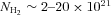 cm−2– i.e. similar to Galactic MCs. The larger X factor values found in lower metallicity systems can be understood due to lower CO abundances (see references in Section 5.4). In molecular-dominated regions such as ULIRGs, the combined effect of higher CO and H2 volume and column densities, higher temperatures (due to enhanced star formation) and larger velocities (due to rotation and/or turbulence) all need to be self-consistently treated to assess the X factor.
We will hereafter refer to 12CO (J=1−0) simply as ‘CO’.
The conversion between  and Σgas includes a factor of 1.4 to account for the mass of helium.
This value is 1.7G0 as determined by Draine (1978), where G0 is the Habing (1968) field.
Since the viewing angle is along the  -axis, vlos= vz. Due to large-scale stochastic variations, the dispersion in vz is not exactly equal to
  .
.
 is not exactly 150 cm−3 because a small fraction of hydrogen remains atomic (Glover & Mac Low 2011).
Though the figures presented here only show the results from one viewing angle (along the  -axis) we have verified that the results are not sensitive to any chosen viewing direction.
We denote any weighted-mean value with 〈…〉, whereas simple averages with an ‘overline’ (e.g.  .)
.)
This saturation brightness temperature is estimated from Fig. 6, which shows the mean values of TBΔv in bins of  . The maximum TB can reach values ≳30 K.
We use the  -component since the CO emission is calculated for the
  -direction.
These LoS velocity dispersions include a contribution from the 0.5 km s−1 microturbulent velocity, so are not exactly equal to  .
.
We are grateful to Desika Narayanan, Alyssa Goodman, Jaime Pineda, Mordecai Mac Low, Erik Rosolowsky and Jerome Pety for useful discussions on CO emission. We also thank the anonymous referee for suggestions that improved our presentation. Several of the simulations reported in this paper were performed on the Ranger cluster at the Texas Advanced Computing Center using time allocated as part of Teragrid project TG-MCA99S024. RSK acknowledges financial support from the Baden-Württemberg Stiftung via their programme International Collaboration II (grant P-LS-SPII/18), and subsidies from the DFG under grants KL1358/10 and KL1358/11, the Sonderforschungsbereich SFB 881. The Milky Way System, as well as from a Frontier grant of Heidelberg University sponsored by the German Excellence Initiative. RS, SCG and RSK are supported by the German Bundesministerium für Bildung und Forschung via the ASTRONET project STAR FORMAT (grant 05A09VHA). This work was supported in part by the US Department of Energy contract no. DE-AC-02-76SF00515. ECO acknowledges support from grant AST 0908185 from the US National Science Foundation.
REFERENCES
Appendices
APPENDIX A: THE EFFECT OF MICROTURBULENCE
As indicated in Section 3 for the radiative transfer calculation, we set the microturbulent velocity vMTRB = 0.5 km s−1 in each zone of the simulation. This value is motivated by loosely extrapolating the observed linewidth–size relationship (Larson 1981; Solomon et al. 1987) down to the physical resolution of the simulation (∼0.1 pc). Due to observational uncertainties and the scatter in the observed linewidth–size relationship, the turbulent velocity at any given scale is not precisely known. We have thus explored how other values of vMTRB may affect our results.
Fig. A1 shows the spectrum from one LoS. It corresponds to LoS B shown in Fig. 15. Three spectra are shown, with different values of vMTRB = 0.25, 0.5 and 0.75 km s−1. With higher microturbulence the line is broadened, and gaps or sharp features in the spectrum can become smooth, as evident near velocities of −0.5 and −5.0 km s−1.
CO spectra from LoS B (see Fig. 15). Three different microturbulent velocities are considered: 0.25 (red), 0.5 (black) and 0.75 (blue) km s−1. The velocity-integrated intensities W are indicated.
The variations in the spectra lead to slight differences in the velocity-integrated intensity W. For vMTRB = 0.25, 0.5 and 0.75 km s−1, W = 58.9, 64.2 and 73.0 K km s−1. The differences in integrated intensity will of course result in corresponding differences in the X factor. For this LoS, the column density is 1.1 × 1022 cm−2, providing X = 1.9, 1.7 and 1.5 × 1020 cm−2 K−1 km−1 s. In the cloud-averaged spectra (e.g. Fig. 17), the smooth Gaussian profiles are not significantly affected, and the linewidths only vary by ≲6 per cent from the fiducial model (e.g. Fig. 17). For vMTRB = 0.25, 0.5 and 0.75, the peak TB, 0 = 5.1, 5.8 and 6.3 K, leading to cloud-averaged X factors 2.6, 2.2, 1.9 × 1020 cm−2 K−1 km−1 s, respectively.
We have found that the precise value of vMTRB does not affect the cloud-averaged spectrum − and the X factor − significantly. The most noticeable difference occurs in the line shapes along individual LoSs. Nevertheless, even then the differences are minimal. Any value of vMTRB within the reasonable range ∈ 0.25–0.75 would produce very similar CO intensities. Thus, the values of the X factor found in this work, and the conclusions drawn from its analysis, would not be affected if different values of vMTRB were employed.
APPENDIX B: NUMERICAL RESOLUTION
While performing radiative transfer calculations, there is a potential for obtaining inaccurate line intensities due to an unresolved velocity structure. In this section, we discuss why resolving the velocity gradients is important, and how we have accounted for under-resolved velocities in our study.
In a grid-based model, the physical properties are only defined in each zone – either at the zone centre or zone edge. While integrating the equation of radiative transfer, or ray-tracing, through a given LoS, the optical depth is only updated when stepping from one grid zone to the next. For a given ‘observed’ frequency ν, corresponding to velocity vobs, the optical depth τν is only modified in zones with LoS velocities that correspond to the non-zero portion of the Gaussian profile function ϕν (see equation 7 and equation 6 in Paper I).
As an example, consider the velocity profile of a sample LoS shown in Fig. B1. The LoS component of the velocity vs is only defined at discrete locations along the LoS s (e.g. edges of grid zones). At the indicated vobs, due to the large velocity gradients, there would be no emission (or, if optically thick, absorption) from this region, since none of the velocities overlap with vobs. Of course, if the (Gaussian) width of ϕν were large enough (e.g. due to microturbulence), then there may be a contribution from one or more zones. For our present discussion, however, we will assume that ϕν has a narrow width (e.g. the vertical extent of the dots defining vs in Fig. B1).
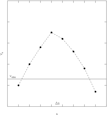
Velocity component along the LoS, vs versus s. A sample-observed frequency (or velocity) is shown by the solid line, vobs. The units of vs and s are arbitrary. Due to the large velocity gradients, there would not be any observed emission at this vobs, unless the velocities were interpolated (dashed line).
In MCs, and generally in any environment, the velocities are not discretized but rather vary continuously throughout the medium. Therefore, the velocities in Fig. B1 are more accurately described by the dashed line connecting the defined vss in each zone. Consequently, at the observed velocity there would in fact be emission along this LoS, due to the overlap of vs and vobs (at two locations in this example).
In order to account for the continuous variation in cloud properties, we have implemented interpolation into our radiative transfer calculations (also see Pontoppidan et al. 2009). All the required quantities, such as temperature, CO density, H2 density and position, are linearly interpolated, effectively increasing the physical resolution along the LoS.
Fig. B2 shows how undersampling the velocities may produce inaccurate line profiles. The figure shows the relevant quantities from LoS A shown in Fig. 15 and discussed in Section 4.5. The left-hand panels show the results using interpolation (16× the original grid, so Δs = 0.0049 pc), and the right-hand panels show the result using the original simulation grid (Δs = 0.078 pc). Clearly, there are stark differences in the spectra. When unresolved, the spectrum has numerous ‘flat tops’, and there is a sharp decrease in the intensities between −3 and −4 km s−1. These features do not occur in the spectrum obtained from the interpolated LoS. The ‘flat tops’ and intensity drop could be misidentified as saturation or absorption features, respectively, when in fact they are simply features arising due to the under-resolved grid.
Spectrum, densities and velocities from LoS A (as in Fig. 15). Top panel shows the brightness temperature (lines – left axis), and integrated optical depth (circles – right axis) as a function of observed velocity. Bottom panels show density (lines – left axis) and LoS velocity (squares – right axis) as a function of LoS position. Left-hand panels show quantities derived using interpolation, and right-hand panels show the quantities derived directly from the original 2563 simulation. The integrated intensities W are indicated in the top panels.
The differences can be understood from the velocity and optical depth profiles. In the high-density region responsible for most of the emission (see Section 4.5), there is a very large velocity gradient. At an observed velocity of −4 km s−1, there would not be any emission from this region, due to the large gap in the velocities at LoS position ∼18.5 pc. However, when interpolated (left-hand panels), there are continuous velocities in this region, resulting in enhanced emission at −4 km s−1.
For the interpolated 0.0049 pc and original 0.078 pc simulations, the integrated intensities from LoS A are 187.1 and 173.8 K km s−1, respectively. This results in a slight difference of ∼10 per cent, and would lead to a similar discrepancy in the X factor from this LoS. The precise difference would of course depend on the particular LoS – LoSs with many regions with large velocity gradients would be strongly affected by under-resolved velocities. For model n300, the cloud-averaged X factor is 〈X〉 = 2.2 × 1020 cm−2 K−1 km−1 s, regardless of whether interpolation is employed. Thus, for the n300 model, only the line shapes along individual LoS are affected by under-resolution, but the velocities are sufficiently resolved for estimating the cloud-averaged integrated intensity.
For the models discussed in Section 4.4 where we have directly modified the velocities to have larger dispersions, there will of course be large velocity gradients in adjacent zones. For these models, we find that interpolation results in more significant differences. Recall that in the altered models, the velocities are replaced in the original grid utilized in the chemo-MHD simulation. The altered velocities on this grid have the chosen dispersions. In the radiative transfer calculations, due to the large velocity gradients, interpolation leads to the addition of numerous values to the velocity data set. In the models with large chosen dispersions in the original grid, this interpolation can potentially lead to a velocity dispersion that is different from the chosen one. For instance, in the σ = 24 and 240 km s−1 models, after interpolation (with 16× increased resolution), the effective velocity dispersion becomes 21 and 205 km s−1, respectively. In both the σ = 24 and 240 km s−1 models, we find that interpolation increases the cloud-averaged W by factors of 2 and 4, respectively, and thereby decreases the X factor by a corresponding amount. As these models are highly artificial to begin with, we do not ensure that all the velocities are well resolved. Nevertheless, qualitatively, we can be sure that increasing the velocity dispersion leads to decreasing the X factor. As we state in Section 5.3, models of real sources with very high dispersions, such as ULIRGs, would have to be well resolved in order to quantify the X factor–σ relationship.
