


Abstract
We examine the velocity structure in the gas associated with H i in the damped Lyα absorption system at redshift z= 1.7764 towards the QSO 1331 + 170 using Arecibo H i 21-cm data, optical spectra from the Keck High Resolution Echelle Spectrograph (HIRES) and European Southern Observatory (ESO) Very Large Telescope (VLT) Ultraviolet and Visual Echelle Spectrograph (UVES), and a previously published Hubble Space Telescope (HST) Space Telescope Imaging Spectrograph (STIS) ultraviolet spectrum. From the optical data we find at least two, and possibly three, components showing C i lines. One of these has very narrow lines with Doppler parameter b= 0.55 km s−1, corresponding to a kinetic temperature of 220 K if the broadening is thermal and with a 2σ upper limit of 480 K. We re-examine the H2 analysis undertaken by Cui et al. using the neutral carbon velocity structure, and find a model which is, unlike theirs, consistent with a mixture of collisional and background radiation excitation of the observed H2 rotational levels. Using Voigt profile fits to absorption lines from a range of singly ionized heavy elements we find eight components covering a velocity range of ∼110 km s−1, with a further outlier over 120 km s−1 away from the nearest in the main group. The H i structure is expected to follow some combination of the singly ionized and neutral gas, but the 21-cm absorption profile is considerably different. We suggest, as have others, that this may be because the different extent and brightness distributions of the radio and optical background sources mean that the sightlines are not the same, and so the spin temperature derived by comparing the Lyα and 21-cm line strengths has little physical meaning. The neutral and singly ionized heavy element line profiles also show significant differences, and so the dominant components in each appear to be physically distinct. Attempts to use the range of atomic masses to separate thermal and turbulent components of their Doppler widths were not generally successful, since there are several blended components and the useful mass range (about a factor of 2) is not very large. The velocity structure in all ionization stages up to +3, apart from the neutral heavy elements, is sufficiently complex that it is difficult to separate out the corresponding velocity components for different ionization levels and determine their column densities.
1 INTRODUCTION
It has long been known that there is significant temperature structure in the interstellar medium (ISM) in the Galaxy. Theoretical models, as originally proposed by e.g. Field, Goldsmith & Habing (1969) and McKee & Ostriker (1977) and refined by several authors subsequently, predict a number of phases in pressure equilibrium. These are a cold neutral medium (CNM), characterized by temperatures T of up to a few 100 K, warm neutral and warm ionized media (WNM and WIM, respectively) with 1000 ≲T≲ 10 000 K and a hot ionized medium (HIM) with T≳ 106 K.
Within the Galaxy, observations of the 21-cm line have led to the detection of hyperfine spin temperatures ∼3000–8000 K, characteristic of the WNM (Carilli, Dwarakanath & Goss 1998; Kanekar et al. 2003). Observations of both the CNM and WNM are described by Heiles & Troland (2003), who give a range of spin temperatures for the cold medium up to ∼200 K, and upper limit kinetic temperatures for the WNM of up to ∼20 000 K. Contrary to the predictions of McKee & Ostriker (1977), a significant fraction of the WNM is at temperatures where the gas is thermally unstable; i.e. T≈ 500–1500 K. On the other hand, direct observational confirmation of the temperatures predicted for a thermally stable WNM have been provided by Redfield & Linsky (2004). They used high-resolution spectra from the Hubble Space Telescope (HST) and compared line profiles from D i with those from heavy elements including Mg ii and Fe ii to obtain local ISM temperatures ∼6500 ± 1500 K. They also noted that the line broadening is not always purely thermal, and that there is a mean bulk flow component within regions of a little over ∼2 km s−1.
For most heavy element quasar absorption systems, the gas is ionized and the kinetic temperature estimates range from ∼104 K up to ∼106 K in some cases where O vi is found. For those with high H i column densities, the damped Lyα systems (DLAs), the gas is clearly neutral, with the heavy elements neutral or singly ionized. However, the ubiquitous presence of C iv and Si iv (Wolfe & Prochaska 2000) and the recent detection of O vi and N v (Fox et al. 2007) absorption indicates that these high-redshift gas layers are also multiphase media. The H i 21-cm spin temperatures provide a means of estimating the thermal conditions in the gas, and generally spin temperatures are measured to be Ts≳ 103 K (see e.g. the compilation by Curran et al. 2005). On the other hand, these estimates assume that the H i column density, N(H i), inferred from the Lyα absorption can be used to compute Ts from the 21-cm optical depth. While this is a straightforward procedure which has been used for the past 30 yr (see Wolfe & Davis 1979), it is complicated by the disparity between the physical sizes of the optical and radio beams subtended by the background quasar at the absorption redshift. Whereas the optical beams are typically less than 1 light-year across, very long baseline interferometry (VLBI) experiments reveal that the radio beams are typically a few hundred parsecs at the low frequencies of the radio absorption lines (e.g. Briggs et al. 1989; Polatidis et al. 1995; Thakkar et al. 1995). Moreover, the appearance of shifts in interferometer phase between the 21-cm line and continuum in VLBI experiments demonstrates a shift in the brightness centroid of the background radio source, which can only be reproduced by a non-uniform distribution of 21-cm opacity towards radio sources with scalelengths of over 200 pc (e.g. Wolfe et al. 1976). For these reasons, the values of Ts inferred by these techniques should be regarded as conservative upper limits.
Temperatures may also be inferred from excitation conditions in other ions and from molecular hydrogen. For example, using measurements of the fine structure levels of Si ii and C ii, Howk, Wolfe & Prochaska (2005) found that the excitation conditions constrain the temperature to T < 954 K in one high-redshift DLA. In those DLAs with H2 absorption, analyses of the relative populations of the lower rotational states give kinetic temperatures, which are generally less than ∼200 K (e.g. Cui et al. 2005; Ledoux, Petitjean & Srianand 2006).
The relationship between excitation temperatures, Tex, and kinetic temperatures, T, depends on the balance between collisional and radiative processes. In DLAs exhibiting 21-cm absorption, the hyperfine excitation temperature, i.e. the spin temperature Ts, likely equals the gas kinetic T because the hyperfine levels are populated mainly by collisions owing to the moderately high densities for the gas, and the long radiative lifetime of the upper (F = 1) hyperfine state. Furthermore, even in regions with low density, ambient Lyα radiation can couple Ts to T via the Field–Wouthuysen effect (e.g. Field 1959). Within the Galaxy, there is good agreement between T and Tex determined from the relative populations of the J = 0 and 1 rotational states of H2, an agreement that holds for column densities log N(H2) ≳ 16 (cm−2). However, excitation temperatures deduced from the relative populations of levels with J≥ 2 depart from T since spontaneous photon emission rates exceed collisional de-excitation rates due to the short radiative lifetimes. Rather the values of Tex inferred for these states are determined by the ambient radiation fields and other processes responsible such as H2 formation on grain surfaces.
In this paper we obtain upper limits to the gas kinetic temperature in neutral regions using the C i absorption lines arising in a DLA at redshift z = 1.776 42 towards the quasar Q1331 + 170. Because this DLA has been detected in 21-cm absorption (Wolfe & Davis 1979), we can compare this temperature with the spin temperature of Ts≳ 1000 K. Also the H2 excitation temperature  K (Cui et al. 2005) has been obtained for this DLA. We shall argue that the true kinetic temperature of some of the gas is at most a few 100 K, and that the value of the spin temperature is likely to be misleading as a result of non-uniform coverage of the background radio source. We also re-examine the physical processes responsible for thermal equilibrium in this DLA and remark on a dilemma not previously discussed. Namely, for a plausible range of volume densities, background radiation alone (Haardt & Madau 2001) will drive Tex≫T. For this reason, the reported H2 level populations in this DLA are difficult to understand. However, adopting the velocity structure inferred from the C i and applying it to the H2 does allow us to produce a physically consistent picture.
We also examine the singly ionized heavy elements, and two more highly ionized species, to look for corresponding structure. This has been done for several objects as part of large DLA surveys e.g. by Prochaska & Wolfe (1999) and Wolfe & Prochaska (2000), with the general conclusion that the singly ionized species structure is similar to that of Al iii, while the component structure of e.g. C iv and singly ionized species bear little relation to each other. We find generally similar results, and show that, for DLA1331 + 170, the fitting of complex velocity structures and associating components across ionization levels is not always straightforward. Consequently there will be uncertainties in the ionization equilibrium models of DLAs (Howk & Sembach 1999). Also, the Al ii/Al iii indicator has been used for the analysis of sub-DLAs (e.g. Dessauges-Zavadsky et al. 2003).
2 OBSERVATIONS
2.1 Radio
The hitherto unpublished radio spectrum was acquired with the Arecibo 300-m telescope of the National Astronomy and Ionosphere Center near Arecibo, Puerto Rico by one of us (AMW) during 1991 April. Because of improvements in receiver technology, the signal-to-noise ratios (S/N values) of the data were significantly improved over the Arecibo discovery spectrum of Wolfe & Davis (1979). The S/N for the data varies between 200 and 400 per 0.7 km s−1 pixel, and the resolution after Hanning smoothing is about 1.4 km s−1.
2.2 Optical
The Keck HIRES (Vogt et al. 1994) spectrum of Q1331 + 170 is the one described by Prochaska & Wolfe (1997). It covers the spectral range from 4220 to 6640 Å at a resolution [full width at half-maximum (FWHM)] of 6.25 km s−1, with a number of gaps at wavelengths >5515 Å. The S/N ∼ 100 per 2 km s−1 pixel at 5400 Å, decreasing to ∼60 in the 4300–4600 Å region.
The Very Large Telescope (VLT) UVES (Dekker et al. 2000) spectrum is based on data available in the European Southern Observatory (ESO) archive in 2006 July. This was obtained with two of the standard echelle settings: on 2002 October 4, for ESO programme 67.A-0022(A), 3 × 4500 s exposures with blue arm central wavelength 346 nm and red arm central wavelength 860 nm, and on 2003 March 12, for ESO programme 68.A-0170(A), 2 × 3600 s exposures with the blue 390/red 564 setting. 2 × 2 on-chip binning was used in both cases. See the VLT UVES handbook1 for more details. The data were extracted and combined using the uves_popler package.2 The combined spectrum covers the range from 3050 to 10 080 Å, with gaps at 4517–4623, 5597–5679, and some more at wavelengths >6650 Å. The resolution is 7 km s−1, and the S/N ∼ 40 per 2.5 km s−1 pixel at 5400 Å. At 4300 Å, S/N ∼ 30, but it is better at shorter wavelengths, ∼35 at 3600 Å.
Voigt profiles convolved with the instrument profile were fitted to the data using the vpfit package,3 version 9.5. In versions 9 and later the model profiles are generated on a finer grid than the data, and in the application here at least nine sample points were required across the intrinsic FWHM of the narrowest line so that the intrinsic line profile was adequately modelled. The convolution with the instrumental profile is done before resampling back to the original pixel scale for direct comparison with the original data, so there should be no numerical problems associated with possible undersampling of the absorption profile which might have arisen with previous versions of the program.
3 H i SPIN TEMPERATURE
While there appears to be some structure in the 21-cm line profile (see Figs 1 and 8), it is at a marginal level. The overall profile is well fitted by a single Gaussian with z = 1.776 4610 ± 0.000 0039, b = 15.7 ± 0.7 km s−1. Integrating over the optical depth of the entire 21-cm feature gives ∫τνdV = 0.93 ± 0.03 km s−1.
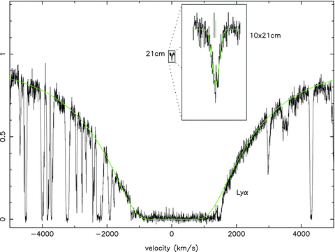
The H i damped Lyα and 21-cm absorption line profiles shown against unit continuum on the same velocity scale relative to a reference redshift z = 1.776 42. The data are shown in black with Voigt profile fit to the damped Lyα at z = 1.776 74 shown in green. The fitted curve departs from the data at longer wavelengths in the base of the damped Lyα line because of the presence of another (sub-DLA) absorption system at z = 1.786 36. The 21-cm line is also shown offset to the right and expanded by a factor of 10 in both x- and y- directions, with a grey tick mark indicating the reference redshift and a green one the fitted line centroid.
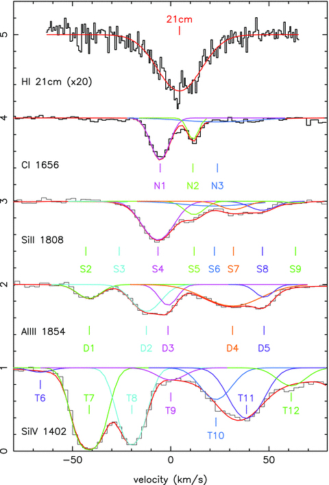
The velocity structure of the H i 21-cm, C i 1656, Si ii 1808, Al iii 1854 and Si iv 1402 absorption lines on a common velocity scale. The total Voigt profile fits are shown in red, and individual components for the various ions shown in colours corresponding to the labels given in Tables 1, 3 and 4.
The H i column density inferred from a Voigt profile fit to the damped Lyα line for the whole complex fitted as a single component (with an additional component in the long wavelength base to allow for the known sub-DLA system at z = 1.786 36) is log N(H i) = 21.17 (cm−2), in agreement with Prochaska & Wolfe (1999) who report log N(H i) = 21.176 ± 0.041. The Lyα and 21-cm profiles are shown on the same velocity scale in Fig. 1. The formal error in our column density value is <0.01, but systematic errors are likely to predominate. Estimates using different continua and blending from other systems gave a range 21.10 < log N(H i) < 21.24, so we adopt 0.07 as an error estimate. The redshift is z = 1.776 74 ± 0.000 09, which is consistent with the 21-cm redshift. If we constrain the Lyα redshift and Doppler parameter to be the same as those for the 21-cm line, then log N(H i) = 21.17.
With this value for the H i column density, the spin temperature Ts = 870 ± 160 K, assuming complete coverage of the absorber. This is consistent with the results of Wolfe & Davis (1979), who give Ts = 980 K, with a lower limit of 770 K. If we take the covering factor estimate f = 0.72 provided by Kanekar et al. (2009), then the corresponding temperature is Ts = 1360 K.
4 NEUTRAL HEAVY ELEMENTS
We first investigate transitions arising from the neutral state of various elements, since these are expected to arise in the CNM phase of the gas. The main lines available in the spectral range covered are from C i and Mg i.
C i in this system has been studied by Songaila et al. (1994), using Keck HIRES spectra of the ground state and fine structure lines in the multiplets at 1656 and 1560 Å to determine excitation temperatures of Tex = 10.4 ± 0.5 for the component at z = 1.776 38, and Tex = 7.4 ± 0.8 at z = 1.776 54. The UVES spectra extend the coverage so that lines at shorter wavelengths, specifically 1328, 1280 and 1277 Å, may also be used to constrain the component parameters. Some of these are blended with lines of other elements at different redshifts, and all lie within the Lyα forest absorption region. We have carefully fitted the C i lines and included possible blends in the fitting procedure, taking advantage of other transitions from these blended lines to help constrain their parameters. Details for each wavelength region used in the fitting procedure are as follows:
C i 1656 falls in a gap in the VLT UVES coverage, and so the fit relies on Keck HIRES data alone. There is blending with weak C iv 1550 at z = 1.966 16 in the blue wing. C iv 1548 at this redshift shows a single component only, so the 1550 line has no significant effect on C i 1656 at z = 1.776 37.
C i 1560 is covered by both the Keck and VLT spectra. It has Al iii 1862 nearby, at z = 1.325 35–1.328 84, and the corresponding Al iii 1854 is blended with C iv 1548 at z = 1.785 86–1.787 19. The corresponding C iv 1550 shows that Al iii blending of C i 1560 is not significant. C i* 1560 is just shortwards of Fe i 2484 at z = 0.744 61, from a well-known system which shows multicomponent Mg ii. Fe i 2523 and 2719 were fitted simultaneously at this redshift, showing a single velocity component which does not affect the C i* lines.
C i 1328 and lines at shorter wavelength have coverage only from UVES at the VLT. The fit to C i 1328 includes a broad weak Lyα at z = 2.035 94, but this changes the effective continuum for the C i* lines mainly. It is much broader than the C i* lines measured. C i** 1329 is in the wing of Lyα at z = 2.036 96, again with small effect on the line parameters.
C i and C i* 1280 are blended with strong Lyα lines at z = 1.923 98–1.924 71. Only the ground state C i 1280 at z = 1.776 37 is well constrained.
C i 1277 is blended with weak Lyα at z = 1.917 45, 1.917 82 and 1.918 37, affecting mainly the C i* and C i** lines with redshifts z > 1.7765 and rest wavelengths >1277.5 Å.
A further complication is that the isotope shifts for 13C i relative to 12C i lines at 1656, 1560 and 1328 Å are, respectively, 0.65, −3.30 and −1.65 km s−1. These will be particularly important where the lines are intrinsically narrow. For this reason 13C i was included as a separate species, with wavelengths and oscillator strengths, for those three lines from Morton (2003). For the other two transitions used to fit the C i, at 1280 and 1277 Å, the spectral S/N is lower so the absence of a 13C i component makes little difference to the final result. We verified this by noting that the removal of 13C i 1328 (where the S/N is higher than for the 1277 or 1280 lines) from the line list had an insignificant effect on the results.
The results of the profile fitting are shown in Fig. 2. A satisfactory fit to the data required the presence of at least three C i velocity components, at velocities of −5.4, 11.3 and 23.8 km s−1 relative to an arbitrarily chosen reference redshift of z = 1.776 42. We henceforth designate these as components N1, N2 and N3, respectively. Details of the fitted parameters for the C i lines, and any others required to fit the data in the regions of those lines, are given in Table 1. 13C i was marginally detected only in the narrow component, N2.
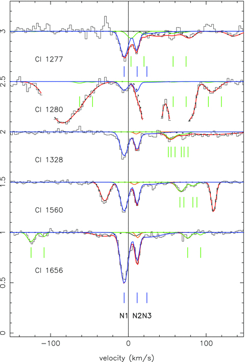
The C i lines on a velocity scale relative to a reference redshift z = 1.776 42. The data are shown in black with Voigt profile fits to C i in dark blue, C i* in green, C i** as dark blue dot–dashed (discernible only for the N1 component in the C i 1656 profile at ∼5 km s−1) and unrelated lines at different redshifts as grey dots. The possible 13C i component is shown in orange. The total fitted profiles are shown in red. The continuum is normalized to unity, and different zero offsets (of an integer × 0.5) have been applied to separate the various transitions. The tick marks show the centroids of the fitted features for the C i components N1, N2 and N3 (see text). The green tick marks indicate the positions for the C i* transitions in each wavelength region.
C i and blends.
| Ion | z | ± | b | ± | log N | ± | Notes |
| Fe i | 0.744 6128 | 0.000 0006 | 1.20 | 0.18 | 12.04 | 0.02 | Fe i 2484 near C i* 1560 |
| Al iii | 1.325 3472 | 0.000 0014 | 6.26 | 0.32 | 12.30 | 0.02 | Al iii 1862 near C i 1560 |
| Al iii | 1.328 1613 | 0.000 0072 | 7.17 | 0.86 | 12.12 | 0.06 | |
| Al iii | 1.328 2625 | 0.000 0048 | 6.22 | 0.78 | 12.21 | 0.05 | |
| Al iii | 1.328 5315 | 0.000 0014 | 11.87 | 0.27 | 12.55 | 0.01 | |
| Al iii | 1.328 8447 | 0.000 0057 | 9.65 | 1.15 | 11.76 | 0.04 | |
| C i | 1.776 3702 | 0.000 0009 | 5.08 | 0.24 | 13.08 | 0.02 | N1 (−5.4 ± 0.1 km s−1) |
| C i* | 1.776 3702 | 5.08 | 12.59 | 0.02 | |||
| C i** | 1.776 3702 | 5.08 | 11.90 | 0.14 | |||
| C i | 1.776 5246 | 0.000 0014 | 0.55 | 0.13 | 13.06 | 0.13 | N2 (11.3 ± 0.2 km s−1) |
| C i* | 1.776 5246 | 0.55 | 12.05 | 0.07 | |||
| C i** | 1.776 5246 | 0.55 | <11.70 | ||||
| 13 C i | 1.776 5246 | 0.53 | 11.78 | 0.28 | |||
| C i | 1.776 6400 | 0.000 0467 | 24.45 | 6.18 | 12.51 | 0.11 | N3 (23.8 ± 5.1 km s−1) |
| C i* | 1.776 6400 | 24.45 | <12.20 | ||||
| C i** | 1.776 6400 | 24.45 | <12.25 | ||||
| C iv | 1.785 8576 | 0.000 0180 | 28.88 | 2.38 | 12.93 | 0.03 | C iv 1550 near Al iii 1854 |
| C iv | 1.786 1859 | 0.000 0117 | 10.49 | 2.06 | 12.43 | 0.13 | |
| C iv | 1.786 4237 | 0.000 0116 | 16.49 | 1.75 | 12.80 | 0.04 | |
| C iv | 1.786 9053 | 0.000 0121 | 14.83 | 1.75 | 12.62 | 0.05 | |
| C iv | 1.787 1942 | 0.000 0187 | 15.63 | 2.70 | 12.47 | 0.07 | |
| H i | 1.917 4518 | 0.000 0518 | 16.90 | 9.29 | 11.93 | 0.23 | Lyα in C i 1277 region |
| H i | 1.917 8188 | 0.000 0201 | 7.20 | 3.74 | 11.86 | 0.16 | |
| H i | 1.918 3670 | 0.000 0841 | 10.65 | 11.33 | 11.86 | 0.43 | |
| ?? | 1.923 8783 | 0.000 0317 | 7.78 | 2.01 | 12.89 | 0.25 | Line in C i 1280 region |
| ?? | 1.923 9821 | 0.000 0106 | 6.60 | 0.93 | 13.23 | 0.11 | |
| H i | 1.924 2860 | 0.000 0042 | 11.48 | 0.71 | 13.32 | 0.03 | |
| ?? | 1.924 3053 | 0.000 0064 | 1.21 | 3.54 | 12.86 | 2.02 | |
| ?? | 1.924 4645 | 0.000 0067 | 2.21 | 2.12 | 12.25 | 0.09 | |
| H i | 1.924 7054 | 0.000 0138 | 9.95 | 2.44 | 12.18 | 0.08 | |
| C iv | 1.966 1609 | 0.000 0093 | 16.53 | 1.57 | 12.47 | 0.04 | C iv 1550 near C i 1656 |
| H i | 2.035 9392 | 0.000 0731 | 37.31 | 12.66 | 12.14 | 0.17 | Lyα in C i 1328 region |
| H i | 2.036 9588 | 0.000 0458 | 19.80 | 7.66 | 12.03 | 0.24 | |
| H i | 2.037 6443 | 0.000 0388 | 55.83 | 9.36 | 12.91 | 0.09 | |
Note: Doppler parameters b are in km s−1, and column densities are log N cm−2. Error estimates are 1σ, and upper limits are 2σ. The C i wavelengths used were those for 12C except where the isotope is given explicitly. Lyα lines with b < 10 km s−1 are probably unidentified heavy elements, and are marked ‘??’. Their parameters were determined assuming that the rest wavelength and oscillator strength are the same as for Lyα. For the C iv and Al iii doublets both lines were included in the fits, and for Fe i at redshift z = 0.774 613 the lines at 2167, 2484 and 2719 were used. Component labels are shown in bold, and the velocities given for the three identified components are relative to a reference redshift z = 1.776 42.
The C i Doppler parameter,  km s−1, for component N1 corresponds, if the broadening is purely thermal, to a temperature of over 16 000 K, so it is likely that bulk motions are the major contributors. We cannot determine if it is a single component with some bulk motion across or within it, or if the apparent width arises because more than one component is present with separations less than the instrument resolution. The populations of the three C i levels are not consistent with a single excitation temperature – the best fit is Tex = 11.24 ± 0.34 K, but the observed C i** column density is then too high relative to the fit by Δlog N = 0.65, i.e. over 4.5σ.
The unresolved C i in component N2 with  0.13 km s−1 has, for thermal line broadening, a kinetic temperature T = 220 K, with a 2σ upper limit T < 480 K. This is much lower than the 21-cm spin temperature for the whole complex, and much higher than the C i*/C i excitation temperature [which, for this component, is 6.90+0.76−0.62 K, in agreement with Songaila et al. (1994) to within the errors].
Component N3 is required only for the strongest two C i lines (at 1560 and 1656 Å). It is very broad, and all we can say from its presence is that there are likely to be a number of weak C i components present over a velocity range of ∼50 km s−1 centred on the redshift given. They do not strongly affect the derived parameters for the two narrower systems.
5 THE NARROW C i COMPONENT
5.1 Doppler width determination and its reliability
The C i lines in component N2 are unresolved, and their profiles in the spectral data are close to the instrument profile, so we should consider further whether or not these Doppler parameters and their error estimates are reliable. If all the lines are unsaturated then the Doppler parameters are not well constrained, as demonstrated by Narayanan et al. (2006). However, it is possible to infer the Doppler parameters for the unblended C i lines to quite good precision provided that not all of the lines are on the linear part of the absorption line curve of growth, as was demonstrated in a similar context by Jorgenson et al. (2009). Strömgren (1948) describes the basic technique as applied to line doublets, and this generalizes to multiple lines, and multiple species. There are many other examples of its use in this way, e.g. Morton (1975), McCandliss (2003) and Cui et al. (2005). For unresolved lines the minimum χ2 profile fitting technique matches the equivalent widths of the lines, and so if there are a number of saturated as well as unsaturated lines present the Doppler parameter b may be determined even where there are possible blends with other components or ions from different redshift systems.
To illustrate how it applies for the narrow C i component discussed here, and to highlight the circumstances under which we may derive reliable Doppler parameters and column densities from unresolved absorption lines, we have generated a new continuum which contains all absorption lines fitted apart from those of component N2 ground state C i. We then determined equivalent widths, with approximate error estimates, for the component N2 C i 1656, 1560, 1328, 1280 and 1277 Å transitions, and show these in Fig. 3 as error ranges on a curve of growth where the C i column density is the best-fitting value from Table 1.
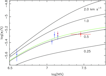
Curves of growth for Doppler parameters b = 0.25, 0.5, 1.0, 2.0 and 4.0 km s−1 (solid lines) and for the component B best-fitting value of b = 0.55 km s−1 (green). Estimated ranges for the equivalent widths w of the C i transitions at rest wavelengths λ = 1656, 1560, 1277, 1328 and 1280 give the w/λ values ordered from right to left. For C i 1560, both the HIRES (red filled circles) and UVES (blue squares) equivalent width ranges are shown. The best estimate column density log N = 13.06 was used to set the x-position, and the error range corresponding to the uncertainty in log N is shown against the 1656 Å line.
It is clear from Fig. 3 that the measured transitions with the highest and the lowest oscillator strengths, i.e. 1656 and 1280, are vital for constraining the Doppler parameter. The free parameter along the x-axis is the C i column density, and had the strongest line, C i 1656, not been measurable (e.g. through blending), then the remaining points adequately fit the curves for any larger Doppler parameter – the C i column density could then be a factor of 2 lower, and the points on the linear part of the curve of growth, and so the Doppler parameter constrained only by the much larger instrument resolution value.
If the weakest line used, C i 1280, had not been measured, then there are much greater uncertainties in the column density, which could then be well over a factor of 10 higher with the consequence that the Doppler parameter would be somewhat lower. This would reduce the temperature upper limit, and make any relative abundance analysis very uncertain.
These may be obvious points to make, but when using automated profile fitting procedures one can forget about their inadequacies, or ignore the large error estimates. It is important to check that the constraints one obtains are based on the data, and not e.g. some approximation made in estimating the errors in the parameters.
The vpfit program provides error estimates from the diagonal terms in the covariance matrix, and these are generally reliable for systems in which the lines are resolved. For systems where the linewidths are considerably less than that of the instrument profile, the reliability of the estimates for the parameters and their errors has been little investigated. We have done so here by generating 84 simulated spectra with the same S/N as the original data using the line parameters given in Table 1. For each of these, Voigt profiles were fitted using the same fitting regions as in the original data, and the resultant parameters compared with those used to generate the spectra.
From these trials, the distribution of both the log column density and Doppler parameters alone shows that there is no significant difference between the input and mean output values. For the column density, the mean and standard deviation are  and s = 0.104, compared with an input value of
  and vpfit error estimate of 0.134. For the Doppler parameter input b = 0.553, with vpfit error 0.125, the mean estimate from the 84 trials is
  , with a standard deviation of 0.082. Therefore the difference between mean values from the simulated spectra differ from the input values by about the estimated error for those means (for the log column densities, the difference is 0.013 and the error estimate is 0.011; for the Doppler parameters the corresponding quantities are 0.009 and 0.008).
From the same trials, we find that the carbon isotope ratio and its error estimate for this component  are reliable. A 2σ lower limit for the 12C/13C ratio is 5.
Further checks were undertaken to verify that there are no additional uncertainties in the analysis of the data.
The stopping criterion for the iterations involved in the fitting process was chosen to be when a change in χ2 < 1.0 × 10⁻⁵. For any search where convergence to the solution is slow, this could result in e.g. the Doppler parameter being biased towards the initial guess relative to the true value. Tests showed this concern to be unfounded for the stopping criterion adopted.
Tests were run to verify that the adopted instrument resolution did not significantly affect the results. It is difficult to see how the resolution in each case could be worse than the slit-limited values which were adopted for the fits described above, but in conditions of good seeing the values of the FWHM appropriate for the spectra could be lower. We attempted to estimate the instrumental resolution by minimizing χ2 for profile fits to the Fe ii 2344, 2374, 2382, 2586 and 2600 Å lines at z = 1.328, and found somewhat broad minima with FWHM ∼ 5.8 km s−1 for both the HIRES and UVES data. Adopting this value yields
 with b = 0.47 ± 0.18 for system N2.
Jenkins & Tripp (2001) have estimated C i oscillator strengths from ISM absorption in early-type stars using HST STIS data. Jenkins (private communication) has also suggested that the C i 1560 oscillator strength, which is given by Morton (2003) as fik = 0.0774, could be as high as fik = 0.1316. Voigt profile fits with the Jenkins & Tripp (2001),f-values give results which differ by only a little from those obtained using the Morton (2003) values, with b = 0.53 ± 0.13 km s−1 and
 , though the χ2 statistic for the fit is now somewhat too high.
From all these trials we conclude that the parameter estimates for system N2 from vpfit, for this mixture of saturated and unsaturated lines, are reliable, though the vpfit error estimates are too high by a factor of ∼1.3–1.5. In particular, the best estimate for the C i Doppler parameter from the trials is  . This corresponds to a temperature of T = 220 K if the broadening is thermal, and in any case the 2σ upper limit to the kinetic temperature for this component is 480 K. Consequently the gas in component N2 is very likely to be a CNM.
5.2 Physical conditions derived from C i
The closeness of the C i excitation temperature 6.90+0.76−0.62 K to the microwave background temperature at the system redshift, TCMB = 2.725(1 +zabs) = 7.57 K, allows us to place an approximate upper limit to the density in the region, assuming that its temperature is significantly higher, since the density must be low enough that collisional processes are unimportant. We find a hydrogen number density nH≲ 3 cm−3. Under these circumstances, if most of the elements are neutral, we can put a lower limit on the size of the cloud by estimating the amount of neutral hydrogen associated with the cloud as follows. Assuming solar relative abundances, [C/H]⊙=−3.61, and therefore,  . Summing over the ground and excited states gives the total
  cm−2, therefore
  cm−2. The cloud must therefore be greater than
  cm = 0.006 pc. This lower limit is sufficiently small that we would, without evidence from H2, be concerned that the C i absorber only partially covers the background source. We believe this is not the case, for the reason given at the end of Section 6.
6 MOLECULAR HYDROGEN
6.1 Results from a single component fit
Further evidence for CNM gas in DLA1331 + 170 stems from the detection of H2 absorption lines at redshift z = 1.776 553 in the Lyman and Werner bands with rest wavelengths from the Lyman limit to ∼1120 Å (Cui et al. 2005). These authors found the rotational level populations between J = 0 and 5 to be consistent with a Boltzmann distribution characterized by a single excitation temperature, Tex = 152 ± 10 K. This differs from the Galaxy ISM where low values of Tex apply for J = 0–2, or J = 1–3, while higher values of Tex apply if higher values of J are considered. The standard interpretation of the ISM results is that for ortho-H2 (odd J) and para-H2 (even J) separately, the rotational states with the lower values of J are collisionally populated which drives Tex towards the kinetic temperature, T, while rotational states with higher values of J are populated both by ultraviolet (UV) pumping and by the formation processes on grain surfaces which leave H2 in the J = 4 state (Spitzer & Zweibel 1974). The radiative processes are dominant at high J-values because radiative self-shielding is less important. As a result, the constant value of Tex in the case of DLA1331 + 170 implies that Tex=T and that collisional processes dominate radiative processes for all of the rotational J levels J = 0–5.
If collisional processes dominate for J = 4 and 5, then we can place a lower limit on the gas density. It must then exceed the critical density ncrit≡AJ, J− 2/qJ, J− 2, where AJ, J− 2 and qJ, J− 2 are the rates of de-excitation due to spontaneous photon decay and collisions through transitions between the J and J− 2 states. For the J = 4 → 2 transition, ncrit must exceed ∼5 × 103 cm−3 when T = 150 K. The gas giving rise to H2 absorption has some fraction of the total N(H i) column density associated with it, so for this region N(H i) ≤1.5 × 1021 cm−2. The corresponding length-scale of a cloud with this volume density is d≤ 0.1 pc, so much less than the size of the optical continuum source of the background quasar, which probably exceeds 0.5 pc. Therefore, unless the gas is in a thin sheet perpendicular to the sightline, the smaller H2 absorbing cloud cannot cover the continuum source, which it must do in order to produce the saturated and damped absorption lines that arise in DLA1331 + 170.
For these reasons Cui et al. (2005) assume that radiative rather than collisional processes govern the population of the rotational states up to J≥ 4. But in that case the similarity between the Tex computed for states with J≥ 4 and J < 4 (where Tex=T) would be a coincidence. To obtain the required level populations, Cui et al. (2005) find that at λ≈ 1000Å, Jν = 6.7 × 10⁻²³ erg cm−2 s−1 Hz−1 sr−1, which they claim is a reasonable value for FUV background radiation at z = 1.77, since if one assumes a frequency dependence of ν−0.5, Jν is in accord with the value of 7.6 × 10⁻²³ erg cm−2 s−1 Hz−1 sr−1 at the Lyman limit inferred from the proximity effect in the Lyα forest. However, the problem with this argument is that a power-law extrapolation across the Lyman limit frequency, while valid for the quasar contribution to the far-ultraviolet (FUV) background, ignores the dominant contribution of Lyman break galaxies at FUV frequencies. According to Haardt & Madau (2001), Jν≈ 3 × 10⁻²⁰ erg cm−2 s−1 Hz−1 sr−1 at λ≈ 1000Å, which is a factor of 500 higher than the Cui et al. (2005) estimate. The effect of the Haardt & Madau (2001) background on the level populations is shown in Fig. 4, which plots the quantity NJ/gJ versus (EJ−E0)/k, where NJ and gJ are the column densities and degeneracies of the Jth rotational state and EJ is the corresponding energy eigenvalue. We show the odd and even J lower level populations at the same excitation temperature since that is what the data indicate, but have not considered processes linking the two.
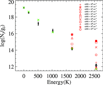
The distribution of H2 over J-levels 0–5. The abscissa is the energy of the level relative to J = 0, and the ordinate is the column density divided by the level degeneracy. The black points with error bars show the Cui et al. (2005) values with error bars, and the green points are the expected values for an excitation temperature of Tex = 150 K. The red points show the expected distribution for a mixture of collisional excitation at this temperature and the Haardt–Madau background radiation at redshift z = 1.7765 for a range of densities log n(H i) = 0–10 (cm−3) as indicated, with the highest points corresponding to the lowest densities.
As a result, our analysis of the H2 absorption lines arising in DLA1331 + 170 has raised the following dilemma. If the J = 0 → 5 rotational states are populated by collisions, then the scalelength of the H2 absorbing gas would be too small. On the other hand, if the rotational states with J≥ 4 are radiatively populated by plausible FUV radiation fields, the predicted values of NJ/gJ would considerably exceed the values inferred from a single H2 cloud model fit.
6.2 Interpreting the H2 data: multiple-component molecular hydrogen
The presence of velocity components N1, N2 and N3 hints at a possible solution to this dilemma; namely, the bulk of the H2 gas resides in the narrow-lined component N2, with the broader components N1 and N3 containing a smaller amount. Consider the evidence. First, our best estimate for the kinetic temperature of component N2, T∼ 200 K (from C i if the line broadening is thermal), is consistent with the H2 excitation temperature, Tex = 152 ± 10 K obtained by Cui et al. (2005). Secondly, the redshift difference between component N2 and H2 absorption, 3.0 km s−1, is less than the difference between H2 and either of the other two C i components. Although the Doppler parameter for the H2 absorption complex, b = 13.9 ± 0.5 km s−1 is considerably greater than that of component N2, we suggest that while component N2 is embedded in the more turbulent medium that dominates the velocity structures of the H2 absorption lines with higher J-values, it none the less contains the bulk of the H2 gas. Consequently, while component N2 is responsible for most of the damping-wing absorption produced for the J = 0 and 1 lines, its low Doppler velocities imply that the absorption from states with higher J-values will be dominated by absorption arising from the more turbulent velocity structures N1 and N3. Stated differently, the values of NJ for J≥ 3 may have been underestimated by the failure to identify the low equivalent widths generated by component N2. As a result, the NJ/gJ versus (EJ−E0)/k curve may in fact be consistent with FUV radiation intensities due to the Haardt & Madau (2001) backgrounds and possibly low rates of local star formation. Finally, it is well known that because C i and H2 are photoionized and photodissociated by photons of similar energy, they are likely to be cospatial and hence show similar velocity structure.
To investigate this possibility further we have performed our own analysis of the Cui et al. (2005) STIS data, assuming a component structure suggested by the C i results. We have taken three components for H2, two at the redshifts corresponding to the C i lines in components N1 and N2. Since the redshift of the third C i component, N3, is not well constrained, the third H2 component redshift (denoted N3′, z = 1.776 7176 ± 0.000 0067) was determined by the profile fitted to the molecular hydrogen lines. The Doppler parameters were constrained so they are physically consistent with those of the corresponding C i, i.e.  , with the limits corresponding to purely turbulent and purely thermal broadening. For the narrow component the adopted Doppler parameter was
  km s−1. The parameters for the profile fits obtained with these constraints are given in Table 2, which also lists the transitions used in the fits. In this case the low J absorption is dominated by component N1, while the higher J is dominated more by the other two velocity components. This is illustrated in Fig. 5 using selected transitions for each J level.
Multicomponent molecular hydrogen column densities.
| Component | N1 | N2 | N3′ | Lines used in fit | |||
| z | 1.776 3702 | 1.776 5246 | 1.776 7176 | ||||
| b (H2) (km s−1) | 8.7 | ±0.5 | 1.0 | – | 10.0 | ±0.7 | |
| log N(J = 0) | 18.56 | ±0.28 | 18.99 | ±0.16 | 15.69 | ±0.63 | 1049, 1077, 1092 |
| log N(J = 1) | 18.90 | ±0.22 | 19.46 | ±0.08 | 17.39 | ±0.40 | 932, 1049, 1051, 1064, 1077,1078, 1092 |
| log N(J = 2) | 16.68 | ±0.24 | 18.44 | ±0.11 | 16.10 | ±0.13 | 927, 987, 1005, 1016, 1051,1053, 1064, 1066, 1079, 1081,1096 |
| log N(J = 3) | 15.94 | ±0.14 | 18.20 | ±0.14 | 16.07 | ±0.14 | 934, 935, 942, 960, 987, 995,997, 1006, 1017, 1041, 1053,1056, 1081, 1096, 1099 |
| log N(J = 4) | 14.95 | ±0.06 | 14.42 | ±0.35 | 14.81 | ±0.06 | 1017, 1035, 1047, 1060, 1074,1085, 1099 |
| log N(J = 5) | 14.46 | ±0.07 | 13.61 | ±0.33 | 14.42 | ±0.07 | 996, 997, 1006, 1017, 1048,1052, 1065, 1079, 1089 |
| Tex(J = 0 and 2) (K) | 86 |  | 177 |  | ≳200 | ||
| Component | N1 | N2 | N3′ | Lines used in fit | |||
| z | 1.776 3702 | 1.776 5246 | 1.776 7176 | ||||
| b (H2) (km s−1) | 8.7 | ±0.5 | 1.0 | – | 10.0 | ±0.7 | |
| log N(J = 0) | 18.56 | ±0.28 | 18.99 | ±0.16 | 15.69 | ±0.63 | 1049, 1077, 1092 |
| log N(J = 1) | 18.90 | ±0.22 | 19.46 | ±0.08 | 17.39 | ±0.40 | 932, 1049, 1051, 1064, 1077,1078, 1092 |
| log N(J = 2) | 16.68 | ±0.24 | 18.44 | ±0.11 | 16.10 | ±0.13 | 927, 987, 1005, 1016, 1051,1053, 1064, 1066, 1079, 1081,1096 |
| log N(J = 3) | 15.94 | ±0.14 | 18.20 | ±0.14 | 16.07 | ±0.14 | 934, 935, 942, 960, 987, 995,997, 1006, 1017, 1041, 1053,1056, 1081, 1096, 1099 |
| log N(J = 4) | 14.95 | ±0.06 | 14.42 | ±0.35 | 14.81 | ±0.06 | 1017, 1035, 1047, 1060, 1074,1085, 1099 |
| log N(J = 5) | 14.46 | ±0.07 | 13.61 | ±0.33 | 14.42 | ±0.07 | 996, 997, 1006, 1017, 1048,1052, 1065, 1079, 1089 |
| Tex(J = 0 and 2) (K) | 86 | | 177 | | ≳200 | ||
Note: column densities are log cm−2. The error estimates are 1σ, and for the (log) column, densities are likely to be underestimates if they exceed ∼0.3. The excitation temperature for component N3′ is effectively unconstrained – a 1σ lower limit is given.
Multicomponent molecular hydrogen column densities.
| Component | N1 | N2 | N3′ | Lines used in fit | |||
| z | 1.776 3702 | 1.776 5246 | 1.776 7176 | ||||
| b (H2) (km s−1) | 8.7 | ±0.5 | 1.0 | – | 10.0 | ±0.7 | |
| log N(J = 0) | 18.56 | ±0.28 | 18.99 | ±0.16 | 15.69 | ±0.63 | 1049, 1077, 1092 |
| log N(J = 1) | 18.90 | ±0.22 | 19.46 | ±0.08 | 17.39 | ±0.40 | 932, 1049, 1051, 1064, 1077,1078, 1092 |
| log N(J = 2) | 16.68 | ±0.24 | 18.44 | ±0.11 | 16.10 | ±0.13 | 927, 987, 1005, 1016, 1051,1053, 1064, 1066, 1079, 1081,1096 |
| log N(J = 3) | 15.94 | ±0.14 | 18.20 | ±0.14 | 16.07 | ±0.14 | 934, 935, 942, 960, 987, 995,997, 1006, 1017, 1041, 1053,1056, 1081, 1096, 1099 |
| log N(J = 4) | 14.95 | ±0.06 | 14.42 | ±0.35 | 14.81 | ±0.06 | 1017, 1035, 1047, 1060, 1074,1085, 1099 |
| log N(J = 5) | 14.46 | ±0.07 | 13.61 | ±0.33 | 14.42 | ±0.07 | 996, 997, 1006, 1017, 1048,1052, 1065, 1079, 1089 |
| Tex(J = 0 and 2) (K) | 86 | | 177 | | ≳200 | ||
Note: column densities are log cm−2. The error estimates are 1σ, and for the (log) column, densities are likely to be underestimates if they exceed ∼0.3. The excitation temperature for component N3′ is effectively unconstrained – a 1σ lower limit is given.
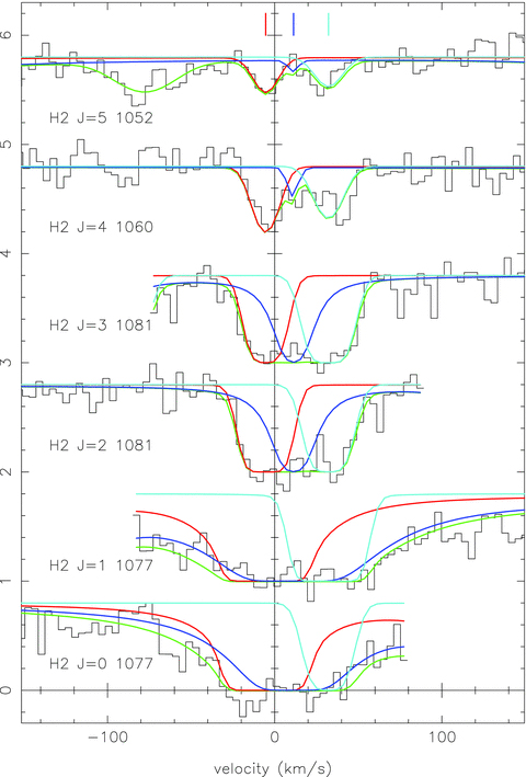
Representative H2 absorption lines from the J = 0–5 levels for the three-component model described in the text. The data are shown in black, the overall fit in green, and the individual contributions from the z = 1.776 3702, 1.776 5246 and 1.776 7176 components in red, blue and turquoise, respectively. The zero-velocity reference is z = 1.776 420, the continuum is set to 0.8 everywhere, and successive lines are offset in y by 1.0. The narrow component (blue) dominates the J = 0 and 1 lines, but is only a minor contributor for J = 4 and 5.
Our three-component fit to the H2 lines is by no means unique, but it does serve to provide a more physically consistent picture of the complex, at least within the rather large errors. The single-component fit giving an apparent single excitation temperature for all excitation levels arises simply because different components dominate different J-values, and is unlikely to reflect the true physical conditions in the individual components.
The molecular hydrogen results also suggest that here, as in the case of Jorgenson et al. (2009), the narrow components inferred for C i are unlikely to be an artefact caused by a small covering factor for the absorbing gas, since the corresponding saturated H2 have zero residual intensities.
7 IONIZED HEAVY ELEMENTS
7.1 Singly ionized species
While DLA1331 + 170 presents clear evidence for the presence of cold gas, it is difficult to determine how much of the neutral hydrogen is associated with it, and so what the overall cold gas fraction of the DLA may be. In an attempt to clarify the overall structure of the DLA we analyse the non-neutral heavy elements.
Some of the H i will be associated with singly ionized heavy elements e.g. C ii, Mg ii, Si ii, Fe ii etc., so that at least part of the component structure of H i will be traced by these ions. For the z = 1.776 42 complex discussed here, the dominant components of all the available lines of C ii and Mg ii are either strongly saturated or too weak to be measurable, so they provide little useful information. For this complex Si ii 1808, S ii 1250 and 1259, Mn ii 2576, Fe ii 1608, 2249 and 2374 and Ni ii 1370, 1709, 1741 and 1751 have the right combination of oscillator strength and column density to be useful, and the saturated lines Si ii 1260, 1304 and 1526 were also used to provide some additional constraints. Some other potentially useful lines were found to be blended with strong lines from other redshift systems, so were omitted from the analysis. All the elements used, with the exception of sulphur, have ionization potentials for i–ii in the range 7.4–8.2 eV, and ii–iii in the range 15.6–18.2 eV, so they should arise predominantly in the same regions. For sulphur, the corresponding potentials are 10.4 and 23.3 eV, so there could be some differences but we failed to find any. For Al ii there is only a single transition available, at 1670 Å, and it was so saturated that the column densities of the dominant components could not be determined.
Since we are interested in physical entities, we have fitted the multiple ions to common redshifts, and constrained the Doppler parameters assuming that bulk motions have a Gaussian distribution, and so the bulk and thermal motions for each ion add in quadrature. Then, for each component,  , where bturb is the turbulent (bulk) component, k Boltzmann’s constant, m the ion mass and T the temperature. In terms of the vpfit program used, this involves fitting bturb and T for at least two ions of different mass at the same redshift simultaneously, with the constraints that both variables are non-negative. The error estimates from the program then apply to bturb and T, not to the Doppler parameters for the individual ions.
From the fitting analysis nine separate velocity components are needed, labelled S1–S9 in increasing redshift order. Details of these are given in Table 3, along with parameters for other systems with lines in the fitting regions used. All the lines fitted were available in the UVES spectrum, and for the HIRES data Fe ii 2249, Si ii 1808, Ni ii 1751 and 1709, Fe ii 1608 and part of Si ii 1526 were included as well. The fitted line profiles and component structure are shown against the UVES data in Figs 6 and 7. An additional component at z = 1.774 8722 was included, since Si ii 1260 from that system is blended with S ii 1259 from the main complex. Its structure was determined using C ii 1334, Mg ii 2796 and 2803, Si ii 1193, 1304 and 1526. Fe ii is not seen in this component, with an upper limit  (cm−2, 2σ).
Singly ionized species and blends.
| Ion | z | ± | b | ± | log N | ± | Sys | Δv (km s−1) | ||
| bturb | ± | T (104K) | ± | |||||||
| C ii | 1.774 8722 | 0.000 0014 | 5.36 | (0.42) | 13.20 | 0.04 | S1 | −167.1 | ||
| Mg ii | 1.774 8722 | 3.76 | (0.28) | 12.11 | 0.01 | 0.0 | 0.9 | 2.1 | 1.1 | |
| Si ii | 1.774 8722 | 3.50 | (0.64) | 12.27 | 0.03 | |||||
| Si ii | 1.776 0202 | 0.000 0039 | 6.46 | 0.52 | 12.70 | 0.03 | S2 | −43.2 ± 0.4 | ||
| Si ii | 1.776 1772 | 0.000 0078 | 5.33 | (0.89) | 13.21 | 0.10 | S3 | −26.2 ± 0.9 | ||
| S ii | 1.776 1772 | 5.20 | (3.50) | 13.44 | 0.13 | 4.3 | 4.2 | 1.7 | 5.8 | |
| Fe ii | 1.776 1772 | 4.82 | (2.23) | 12.46 | 0.14 | |||||
| Si ii | 1.776 3599 | 0.000 0013 | 9.53 | (0.24) | 15.07 | 0.01 | S4 | −6.5 ± 0.2 | ||
| S ii | 1.776 3599 | 9.53 | (0.48) | 14.86 | 0.01 | 9.5 | 0.4 | 0.0 | 1.3 | |
| Mn ii | 1.776 3599 | 9.53 | (1.08) | 12.16 | 0.03 | |||||
| Fe ii | 1.776 3599 | 9.53 | (0.26) | 14.30 | 0.02 | |||||
| Ni ii | 1.776 3599 | 9.53 | (0.73) | 13.10 | 0.03 | |||||
| Si ii | 1.776 5303 | 0.000 0028 | 5.67 | (0.99) | 14.35 | 0.09 | S5 | 11.9 ± 0.3 | ||
| S ii | 1.776 5303 | 5.67 | (1.02) | 14.32 | 0.10 | 5.7 | 4.1 | 0.0 | 0.6 | |
| Fe ii | 1.776 5303 | 5.67 | (3.80) | 13.07 | 0.27 | |||||
| Ni ii | 1.776 5303 | 5.67 | – | 11.43 | 1.01 | |||||
| Si ii | 1.776 6255 | 0.000 0297 | 22.78 | (2.34) | 14.38 | 0.18 | S6 | 22.2 ± 3.2 | ||
| S ii | 1.776 6255 | 22.77 | – | 13.73 | 0.79 | 22.6 | 4.7 | 1.1 | 39 | |
| Mn ii | 1.776 6255 | 22.72 | (15.29) | 12.00 | 0.06 | |||||
| Fe ii | 1.776 6255 | 22.71 | (6.51) | 13.99 | 0.08 | |||||
| Ni ii | 1.776 6255 | 22.71 | (9.38) | 12.98 | 0.08 | |||||
| Si ii | 1.776 7156 | 0.000 0043 | 8.11 | (1.53) | 14.23 | 0.12 | S7 | 31.9 ± 0.5 | ||
| S ii | 1.776 7156 | 7.66 | (2.04) | 14.03 | 0.16 | 3.1 | 4.2 | 9.5 | 6.6 | |
| Fe ii | 1.776 7156 | 6.14 | (1.46) | 13.52 | 0.11 | |||||
| Ni ii | 1.776 7156 | 6.03 | (3.70) | 12.33 | 0.15 | |||||
| Si ii | 1.776 8523 | 0.000 0029 | 8.00 | (0.55) | 14.27 | 0.03 | S8 | 46.7 ± 0.3 | ||
| S ii | 1.776 8523 | 7.97 | (2.53) | 13.99 | 0.07 | 7.7 | 0.8 | 0.8 | 2.0 | |
| Mn ii | 1.776 8523 | 7.86 | (6.00) | 11.51 | 0.13 | |||||
| Fe ii | 1.776 8523 | 7.86 | (0.67) | 13.87 | 0.04 | |||||
| Ni ii | 1.776 8523 | 7.85 | (1.82) | 12.72 | 0.05 | |||||
| Si ii | 1.777 0083 | 0.000 0030 | 4.01 | (0.42) | 13.32 | 0.04 | S9 | 63.5 ± 0.3 | ||
| Fe ii | 1.777 0083 | 3.85 | (1.48) | 12.76 | 0.09 | 3.7 | 2.0 | 0.4 | 2.4 | |
| H i | 1.875 7384 | 0.000 0243 | 23.39 | 0.94 | 14.33 | 0.09 | ||||
| H i | 1.877 5792 | 0.000 0028 | 35.60 | 0.48 | 14.03 | 0.01 | ||||
| H i | 1.876 0396 | 0.000 1075 | 17.46 | 6.86 | 13.25 | 0.53 | ||||
| H i | 1.977 9551 | 0.000 0061 | 21.84 | 0.88 | 12.97 | 0.01 | ||||
| H i | 1.979 9652 | 0.000 0161 | 26.69 | 2.63 | 12.70 | 0.03 | ||||
| ?? | 2.673 7241 | 0.000 0526 | 49.43 | 5.17 | 12.73 | 0.06 | ||||
Note: component labels are given in bold. Error estimates are 1σ, and those in parentheses are indicative Doppler parameter errors if the ion were treated without reference to others in the system (see text for details). Other details are as for Table 1.
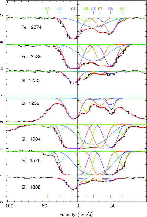
The singly ionized complex centred on redshift z = 1.776 420 showing the total fits in red. These include unrelated blends and the component structure for the lines in the complex. Component velocities and labels (see Table 3) are marked in the corresponding colours. The continuum level is set at 0.9 and each line biased up by an integer amount to separate them. Fe ii 2586 was not included in the fitted regions because of the possibility that the weak structure seen in the blue wing may extend into the line itself, but is shown here as an example of the consistency of the fit obtained using other lines. The dark grey component shown in the S ii 1259 profile is Si ii 1260 at z = 1.774 8722.
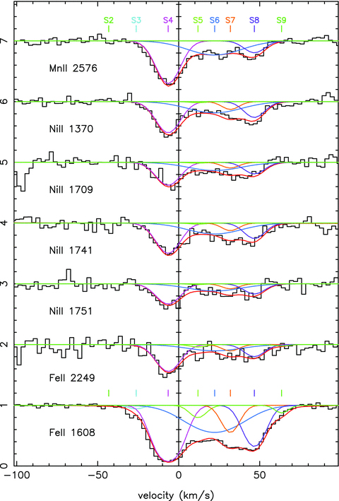
The singly ionized complex centred on redshift z = 1.776 420 showing the total fits in red and the component structure for the lines in the complex for the weaker lines. Component velocities and labels (see Table 3) are marked in the corresponding colours. The continuum and zero level for Fe ii 1608 are unity and zero, as shown, but for the other lines the vertical scale has been stretched by a factor of 4, so the zero levels are four units below the continuum which has been biased upwards in each case by an integer amount to separate the lines.
The component structure given in Table 3 is somewhat different from that given by Prochaska & Wolfe (1997), who illustrate a fitted profile to the Si ii 1808 line. A large part of the difference probably comes about because we have used the additional UVES spectrum and fitted many transitions where they used just one.
For determining which ions provide the strongest constraints it can be useful to have Doppler parameter error estimates for individual ions rather than those for the variables bturb and T. Indicative values are given Table 3. Here the error estimates given for the individual Doppler parameters for each ion were computed by assuming that the best-fitting b-value is the tied one, but computing the errors as if the tied constraint were not applied. In some cases the error exceeded the Doppler parameter, so there is no useful constraint. These are indicated by a dash in the table.
As can be seen from Table 3, for the component structure inferred here, bulk motions dominate in several cases. These are S3, S4, S5, S6, S8 and S9, where the Doppler parameters have similar values for all ions. For S1 and S7, however, thermal broadening is more important, though the temperature estimate for S7, at 95 000 K, is somewhat higher than we might expect. There are several components across the velocity range, and so, partly because most of the systems are now blended and partly because the mass range over which reliable Doppler parameters can be obtained is at most from 28Si to 56Fe, i.e. a factor of less than 2, the error estimates for both bturb and T are rather large. For component S7, the 1σ error estimate is almost 70 000 K, so within the errors the temperature could be only a few × 104 K.
Most temperature errors are smaller, and in two cases (S4 and S5) the 2σ upper limit indicates temperatures of ∼2 × 10⁴ K or less. In general, the temperatures are at least consistent with the notion that the material is in the WNM with temperatures of ∼1–3 × 10⁴ K. However, the errors are large, and so CNM gas is an equally viable interpretation.
7.2 More highly ionized heavy elements
We may explore the structure of more highly ionized species, though, because they have a range of ionization potentials, we cannot necessarily treat them as coming predominantly from the same physical regions. The motivation for doing this is to check whether or not comparison of the column densities of close ions, such as Al ii and Al iii, provides a reliable indicator of the ionization state of the gas.
The doubly ionized species detected in our observed range are Si iii 1206 and Al iii 1854 and 1862. Si iii has only a single line which is saturated, in the Lyα forest and close to the strong damped Lyα associated with the system, so it provides little useful information. Fe iii 1122 is potentially observable, but in a region in the Lyα forest (<3120A) where the S/N in the data is poor. Consequently, we have used only the Al iii doublet to investigate the component structure here. The results are given in Table 4, and the component structure shown against other ions in Fig. 8.
Al iii and Si iv absorption.
| Ion | z | ± |  | ± | log N | ± | Sys | Δv (km s−1) |
| Al iii | 1.776 0362 | 0.000 0047 | 7.12 | 0.95 | 11.99 | 0.04 | D1 | −41.5 ± 0.5 |
| Al iii | 1.776 3051 | 0.000 0172 | 8.93 | 1.56 | 12.40 | 0.11 | D2 | −12.4 ± 1.9 |
| Al iii | 1.776 4071 | 0.000 0098 | 4.74 | 1.69 | 12.08 | 0.21 | D3 | −1.4 ± 1.1 |
| Al iii | 1.776 7114 | 0.000 0107 | 18.85 | 1.41 | 12.57 | 0.04 | D4 | 31.5 ± 1.2 |
| Al iii | 1.776 8598 | 0.000 0052 | 4.56 | 1.67 | 11.83 | 0.13 | D5 | 47.5 ± 0.6 |
| Si iv | 1.774 8504 | 0.000 0012 | 6.62 | 0.16 | 13.36 | 0.01 | T1 | −169.53 |
| Si iv | 1.775 0657 | 0.000 0223 | 10.35 | 3.50 | 12.81 | 0.36 | T2 | −146.27 |
| Si iv | 1.775 0956 | 0.000 0062 | 1.30 | 1.03 | 12.39 | 0.14 | T3 | −143.04 |
| Si iv | 1.775 2779 | 0.000 1684 | 23.70 | 10.30 | 12.77 | 0.48 | T4 | −123.34 |
| Si iv | 1.775 2931 | 0.000 0043 | 5.12 | 1.13 | 12.71 | 0.12 | T5 | −121.71 |
| Si iv | 1.775 8053 | 0.000 0093 | 6.25 | 1.92 | 11.89 | 0.08 | T6 | −66.4 ± 1.0 |
| Si iv | 1.776 0357 | 0.000 0012 | 6.82 | 0.22 | 13.90 | 0.03 | T7 | −41.5 ± 0.1 |
| Si iv | 1.776 2370 | 0.000 0014 | 6.52 | 0.30 | 13.63 | 0.02 | T8 | −19.8 ± 0.2 |
| Si iv | 1.776 4205 | 0.000 0098 | 8.94 | 3.32 | 12.47 | 0.14 | T9 | 0.1 ± 1.1 |
| Si iv | 1.776 6329 | 0.000 0282 | 9.42 | 2.71 | 12.97 | 0.25 | T10 | 23.0 ± 3.0 |
| Si iv | 1.776 7771 | 0.000 0166 | 10.16 | 1.95 | 13.29 | 0.12 | T11 | 38.6 ± 1.8 |
| Si iv | 1.776 9879 | 0.000 0085 | 8.97 | 2.69 | 12.66 | 0.31 | T12 | 61.3 ± 0.9 |
| Si iv | 1.777 3069 | 0.000 0041 | 10.41 | 1.65 | 13.29 | 0.21 | T13 | 95.8 |
| Si iv | 1.777 3179 | 0.000 0567 | 29.11 | 50.81 | 12.96 | 0.18 | T14 | 96.9 |
| Si iv | 1.777 4448 | 0.000 0038 | 2.17 | 1.05 | 12.59 | 0.08 | T15 | 110.6 |
| Si iv | 1.777 6712 | 0.000 0063 | 5.84 | 1.77 | 12.52 | 0.20 | T16 | 135.1 |
| Si iv | 1.777 8277 | 0.000 0541 | 15.81 | 5.97 | 12.40 | 0.33 | T17 | 152.0 |
| Ion | z | ± | | ± | log N | ± | Sys | Δv (km s−1) |
| Al iii | 1.776 0362 | 0.000 0047 | 7.12 | 0.95 | 11.99 | 0.04 | D1 | −41.5 ± 0.5 |
| Al iii | 1.776 3051 | 0.000 0172 | 8.93 | 1.56 | 12.40 | 0.11 | D2 | −12.4 ± 1.9 |
| Al iii | 1.776 4071 | 0.000 0098 | 4.74 | 1.69 | 12.08 | 0.21 | D3 | −1.4 ± 1.1 |
| Al iii | 1.776 7114 | 0.000 0107 | 18.85 | 1.41 | 12.57 | 0.04 | D4 | 31.5 ± 1.2 |
| Al iii | 1.776 8598 | 0.000 0052 | 4.56 | 1.67 | 11.83 | 0.13 | D5 | 47.5 ± 0.6 |
| Si iv | 1.774 8504 | 0.000 0012 | 6.62 | 0.16 | 13.36 | 0.01 | T1 | −169.53 |
| Si iv | 1.775 0657 | 0.000 0223 | 10.35 | 3.50 | 12.81 | 0.36 | T2 | −146.27 |
| Si iv | 1.775 0956 | 0.000 0062 | 1.30 | 1.03 | 12.39 | 0.14 | T3 | −143.04 |
| Si iv | 1.775 2779 | 0.000 1684 | 23.70 | 10.30 | 12.77 | 0.48 | T4 | −123.34 |
| Si iv | 1.775 2931 | 0.000 0043 | 5.12 | 1.13 | 12.71 | 0.12 | T5 | −121.71 |
| Si iv | 1.775 8053 | 0.000 0093 | 6.25 | 1.92 | 11.89 | 0.08 | T6 | −66.4 ± 1.0 |
| Si iv | 1.776 0357 | 0.000 0012 | 6.82 | 0.22 | 13.90 | 0.03 | T7 | −41.5 ± 0.1 |
| Si iv | 1.776 2370 | 0.000 0014 | 6.52 | 0.30 | 13.63 | 0.02 | T8 | −19.8 ± 0.2 |
| Si iv | 1.776 4205 | 0.000 0098 | 8.94 | 3.32 | 12.47 | 0.14 | T9 | 0.1 ± 1.1 |
| Si iv | 1.776 6329 | 0.000 0282 | 9.42 | 2.71 | 12.97 | 0.25 | T10 | 23.0 ± 3.0 |
| Si iv | 1.776 7771 | 0.000 0166 | 10.16 | 1.95 | 13.29 | 0.12 | T11 | 38.6 ± 1.8 |
| Si iv | 1.776 9879 | 0.000 0085 | 8.97 | 2.69 | 12.66 | 0.31 | T12 | 61.3 ± 0.9 |
| Si iv | 1.777 3069 | 0.000 0041 | 10.41 | 1.65 | 13.29 | 0.21 | T13 | 95.8 |
| Si iv | 1.777 3179 | 0.000 0567 | 29.11 | 50.81 | 12.96 | 0.18 | T14 | 96.9 |
| Si iv | 1.777 4448 | 0.000 0038 | 2.17 | 1.05 | 12.59 | 0.08 | T15 | 110.6 |
| Si iv | 1.777 6712 | 0.000 0063 | 5.84 | 1.77 | 12.52 | 0.20 | T16 | 135.1 |
| Si iv | 1.777 8277 | 0.000 0541 | 15.81 | 5.97 | 12.40 | 0.33 | T17 | 152.0 |
Note: error estimates are 1σ. The velocities Δv are relative to a reference redshift z = 1.776 42. See Table 1 for further details.
Al iii and Si iv absorption.
| Ion | z | ± | | ± | log N | ± | Sys | Δv (km s−1) |
| Al iii | 1.776 0362 | 0.000 0047 | 7.12 | 0.95 | 11.99 | 0.04 | D1 | −41.5 ± 0.5 |
| Al iii | 1.776 3051 | 0.000 0172 | 8.93 | 1.56 | 12.40 | 0.11 | D2 | −12.4 ± 1.9 |
| Al iii | 1.776 4071 | 0.000 0098 | 4.74 | 1.69 | 12.08 | 0.21 | D3 | −1.4 ± 1.1 |
| Al iii | 1.776 7114 | 0.000 0107 | 18.85 | 1.41 | 12.57 | 0.04 | D4 | 31.5 ± 1.2 |
| Al iii | 1.776 8598 | 0.000 0052 | 4.56 | 1.67 | 11.83 | 0.13 | D5 | 47.5 ± 0.6 |
| Si iv | 1.774 8504 | 0.000 0012 | 6.62 | 0.16 | 13.36 | 0.01 | T1 | −169.53 |
| Si iv | 1.775 0657 | 0.000 0223 | 10.35 | 3.50 | 12.81 | 0.36 | T2 | −146.27 |
| Si iv | 1.775 0956 | 0.000 0062 | 1.30 | 1.03 | 12.39 | 0.14 | T3 | −143.04 |
| Si iv | 1.775 2779 | 0.000 1684 | 23.70 | 10.30 | 12.77 | 0.48 | T4 | −123.34 |
| Si iv | 1.775 2931 | 0.000 0043 | 5.12 | 1.13 | 12.71 | 0.12 | T5 | −121.71 |
| Si iv | 1.775 8053 | 0.000 0093 | 6.25 | 1.92 | 11.89 | 0.08 | T6 | −66.4 ± 1.0 |
| Si iv | 1.776 0357 | 0.000 0012 | 6.82 | 0.22 | 13.90 | 0.03 | T7 | −41.5 ± 0.1 |
| Si iv | 1.776 2370 | 0.000 0014 | 6.52 | 0.30 | 13.63 | 0.02 | T8 | −19.8 ± 0.2 |
| Si iv | 1.776 4205 | 0.000 0098 | 8.94 | 3.32 | 12.47 | 0.14 | T9 | 0.1 ± 1.1 |
| Si iv | 1.776 6329 | 0.000 0282 | 9.42 | 2.71 | 12.97 | 0.25 | T10 | 23.0 ± 3.0 |
| Si iv | 1.776 7771 | 0.000 0166 | 10.16 | 1.95 | 13.29 | 0.12 | T11 | 38.6 ± 1.8 |
| Si iv | 1.776 9879 | 0.000 0085 | 8.97 | 2.69 | 12.66 | 0.31 | T12 | 61.3 ± 0.9 |
| Si iv | 1.777 3069 | 0.000 0041 | 10.41 | 1.65 | 13.29 | 0.21 | T13 | 95.8 |
| Si iv | 1.777 3179 | 0.000 0567 | 29.11 | 50.81 | 12.96 | 0.18 | T14 | 96.9 |
| Si iv | 1.777 4448 | 0.000 0038 | 2.17 | 1.05 | 12.59 | 0.08 | T15 | 110.6 |
| Si iv | 1.777 6712 | 0.000 0063 | 5.84 | 1.77 | 12.52 | 0.20 | T16 | 135.1 |
| Si iv | 1.777 8277 | 0.000 0541 | 15.81 | 5.97 | 12.40 | 0.33 | T17 | 152.0 |
Note: error estimates are 1σ. The velocities Δv are relative to a reference redshift z = 1.776 42. See Table 1 for further details.
Similarly we can investigate the structure of triply ionized species, such as Si iv and C iv through their doublet absorption lines. In this case we choose Si iv only, since its ionization potential (45.1 eV) is less than that of He ii (54.4 eV), whereas that of C iv (64.5 eV) is above the He ii value, and therefore the two species may not be predominantly in the same regions. The Prochaska & Wolfe (1999) and Wolfe & Prochaska (2000) studies also show that while there is a general similarity in the Si iv and C iv velocity structure, the correspondence is not perfect. The results for the Voigt profile fits to the Si iv 1393 and 1402 doublet are given in Table 4.
8 COMPARING THE VARIOUS COMPONENTS
8.1 Comparing profiles
Fig. 8 shows the H i 21-cm profile with representative lines from neutral, singly and more highly ionized heavy elements. This is quite instructive, since there are some features which may be common to more than one ionization level and others which seem to correspond less well.
The H i 21-cm profile stands out as having little in common with any of the others. While we have no direct measure of what the velocity distribution of the damped Lyα absorption is from the UVES spectrum, if the heavy element abundances are not too disparate between velocity components it would be surprising if it did not roughly follow that of the higher column density heavy element neutral and singly ionized species. Therefore we expect it to follow S4–S8 reasonably well, with some contribution from N1 and N2.
The H i 21-cm line is broad and, at the S/N available, smooth, and is consistent with the absorption arising in a single cloud at a temperature of T = 15 000 K. The difference in shape from that expected from the heavy elements, and the redshift of the maximum absorption from any of the components, make it difficult to escape the conclusion that it and the Lyα absorption have little to do with each other. This reinforces the notion, raised in the context of other objects by Curran et al. (2007) and Kanekar et al. (2009), that the 21-cm and Lyα absorption lines do not arise in the same region(s), possibly because the radio source is extended and so it and the optical source are not coincident. Consequently the derivation of a spin temperature by using the radio 21-cm and the optical Lyα lines may well be inappropriate.
The various ionization stages of the heavy element lines show considerable overlap, especially for the lower ionization states. However, from Voigt profile fitting each ionization stage independently, it is not always clear for adjacent ionization levels what velocity structure they have in common. This is most readily seen from Fig. 8, with details of redshift and Doppler parameters in Tables 1, 3 and 4. Comparative details extracted from these tables are given, in redshift order, in Table 5. In this table we have chosen Si ii as the representative of the singly ionized components, since the silicon and aluminium atomic masses are close in value and so the Doppler parameters of any cospatial components should be nearly the same.
Velocity components compared.
| Ion | z | ± |  | ± | log N | ± | Sys | Δv (km s−1) | |
| Si iv | 1.775 8053 | 0.000 0093 | 6.25 | 1.92 | 11.89 | 0.08 | T6 | −66.4 ± 1.0 | |
| Si ii | 1.776 0202 | 0.000 0039 | 6.46 | 0.52 | 12.70 | 0.03 | S2 | −43.2 ± 0.4 | |
| Al iii | 1.776 0362 | 0.000 0047 | 7.12 | 0.95 | 11.99 | 0.04 | D1 | −41.5 ± 0.5 | ⌉ |
| Si iv | 1.776 0357 | 0.000 0012 | 6.82 | 0.22 | 13.90 | 0.03 | T7 | −41.5 ± 0.1 | ⌋ |
| Si ii | 1.776 1772 | 0.000 0078 | 5.33 | 0.89 | 13.21 | 0.10 | S3 | −26.2 ± 0.9 | |
| Si iv | 1.776 2370 | 0.000 0014 | 6.52 | 0.30 | 13.63 | 0.02 | T8 | −19.8 ± 0.2 | |
| Al iii | 1.776 3051 | 0.000 0172 | 8.93 | 1.56 | 12.40 | 0.11 | D2 | −12.4 ± 1.9 | |
| Si ii | 1.776 3599 | 0.000 0013 | 9.53 | 0.24 | 15.07 | 0.01 | S4 | −6.5 ± 0.2 | |
| C i | 1.776 3702 | 0.000 0009 | 5.08 | 0.24 | 13.08 | 0.02 | N1 | −5.4 ± 0.1 | |
| Al iii | 1.776 4071 | 0.000 0098 | 4.74 | 1.69 | 12.08 | 0.21 | D3 | −1.4 ± 1.1 | ⌉ |
| Si iv | 1.776 4205 | 0.000 0098 | 8.94 | 3.32 | 12.47 | 0.14 | T9 | 0.1 ± 1.1 | ⌋ |
| C i | 1.776 5246 | 0.000 0014 | 0.55 | 0.13 | 13.06 | 0.13 | N2 | 11.3 ± 0.2 | |
| Si ii | 1.776 5303 | 0.000 0028 | 5.67 | 0.99 | 14.35 | 0.09 | S5 | 11.9 ± 0.3 | |
| Si ii | 1.776 6255 | 0.000 0297 | 22.78 | 2.34 | 14.38 | 0.18 | S6 | 22.2 ± 3.2 | ⌉ |
| Si iv | 1.776 6329 | 0.000 0282 | 9.42 | 2.71 | 12.97 | 0.25 | T10 | 23.0 ± 3.0 | |
| C i | 1.776 6400 | 0.000 0467 | 24.45 | 6.18 | 12.51 | 0.11 | N3 | 23.8 ± 5.1 | ⌋ |
| Al iii | 1.776 7114 | 0.000 0107 | 18.85 | 1.41 | 12.57 | 0.04 | D4 | 31.5 ± 1.2 | |
| Si ii | 1.776 7156 | 0.000 0043 | 8.11 | 1.53 | 14.23 | 0.12 | S7 | 31.9 ± 0.5 | |
| Si iv | 1.776 7771 | 0.000 0166 | 10.16 | 1.95 | 13.29 | 0.12 | T11 | 38.6 ± 1.8 | |
| Si ii | 1.776 8523 | 0.000 0029 | 8.00 | 0.55 | 14.27 | 0.03 | S8 | 46.7 ± 0.3 | ⌉ |
| Al iii | 1.776 8598 | 0.000 0052 | 4.56 | 1.67 | 11.83 | 0.13 | D5 | 47.5 ± 0.6 | ⌋ |
| Si iv | 1.776 9879 | 0.000 0085 | 8.97 | 2.69 | 12.66 | 0.31 | T12 | 61.3 ± 0.9 | |
| Si ii | 1.777 0083 | 0.000 0030 | 4.01 | 0.42 | 13.32 | 0.04 | S9 | 63.5 ± 0.3 |
| Ion | z | ± | | ± | log N | ± | Sys | Δv (km s−1) | |
| Si iv | 1.775 8053 | 0.000 0093 | 6.25 | 1.92 | 11.89 | 0.08 | T6 | −66.4 ± 1.0 | |
| Si ii | 1.776 0202 | 0.000 0039 | 6.46 | 0.52 | 12.70 | 0.03 | S2 | −43.2 ± 0.4 | |
| Al iii | 1.776 0362 | 0.000 0047 | 7.12 | 0.95 | 11.99 | 0.04 | D1 | −41.5 ± 0.5 | ⌉ |
| Si iv | 1.776 0357 | 0.000 0012 | 6.82 | 0.22 | 13.90 | 0.03 | T7 | −41.5 ± 0.1 | ⌋ |
| Si ii | 1.776 1772 | 0.000 0078 | 5.33 | 0.89 | 13.21 | 0.10 | S3 | −26.2 ± 0.9 | |
| Si iv | 1.776 2370 | 0.000 0014 | 6.52 | 0.30 | 13.63 | 0.02 | T8 | −19.8 ± 0.2 | |
| Al iii | 1.776 3051 | 0.000 0172 | 8.93 | 1.56 | 12.40 | 0.11 | D2 | −12.4 ± 1.9 | |
| Si ii | 1.776 3599 | 0.000 0013 | 9.53 | 0.24 | 15.07 | 0.01 | S4 | −6.5 ± 0.2 | |
| C i | 1.776 3702 | 0.000 0009 | 5.08 | 0.24 | 13.08 | 0.02 | N1 | −5.4 ± 0.1 | |
| Al iii | 1.776 4071 | 0.000 0098 | 4.74 | 1.69 | 12.08 | 0.21 | D3 | −1.4 ± 1.1 | ⌉ |
| Si iv | 1.776 4205 | 0.000 0098 | 8.94 | 3.32 | 12.47 | 0.14 | T9 | 0.1 ± 1.1 | ⌋ |
| C i | 1.776 5246 | 0.000 0014 | 0.55 | 0.13 | 13.06 | 0.13 | N2 | 11.3 ± 0.2 | |
| Si ii | 1.776 5303 | 0.000 0028 | 5.67 | 0.99 | 14.35 | 0.09 | S5 | 11.9 ± 0.3 | |
| Si ii | 1.776 6255 | 0.000 0297 | 22.78 | 2.34 | 14.38 | 0.18 | S6 | 22.2 ± 3.2 | ⌉ |
| Si iv | 1.776 6329 | 0.000 0282 | 9.42 | 2.71 | 12.97 | 0.25 | T10 | 23.0 ± 3.0 | |
| C i | 1.776 6400 | 0.000 0467 | 24.45 | 6.18 | 12.51 | 0.11 | N3 | 23.8 ± 5.1 | ⌋ |
| Al iii | 1.776 7114 | 0.000 0107 | 18.85 | 1.41 | 12.57 | 0.04 | D4 | 31.5 ± 1.2 | |
| Si ii | 1.776 7156 | 0.000 0043 | 8.11 | 1.53 | 14.23 | 0.12 | S7 | 31.9 ± 0.5 | |
| Si iv | 1.776 7771 | 0.000 0166 | 10.16 | 1.95 | 13.29 | 0.12 | T11 | 38.6 ± 1.8 | |
| Si ii | 1.776 8523 | 0.000 0029 | 8.00 | 0.55 | 14.27 | 0.03 | S8 | 46.7 ± 0.3 | ⌉ |
| Al iii | 1.776 8598 | 0.000 0052 | 4.56 | 1.67 | 11.83 | 0.13 | D5 | 47.5 ± 0.6 | ⌋ |
| Si iv | 1.776 9879 | 0.000 0085 | 8.97 | 2.69 | 12.66 | 0.31 | T12 | 61.3 ± 0.9 | |
| Si ii | 1.777 0083 | 0.000 0030 | 4.01 | 0.42 | 13.32 | 0.04 | S9 | 63.5 ± 0.3 |
Note: component labels are given in bold. Systems which may be associated are grouped between horizontal lines, and those for which the redshifts and Doppler parameters are compatible are shown linked with a right bracket. See Table 1 for other details.
Velocity components compared.
| Ion | z | ± | | ± | log N | ± | Sys | Δv (km s−1) | |
| Si iv | 1.775 8053 | 0.000 0093 | 6.25 | 1.92 | 11.89 | 0.08 | T6 | −66.4 ± 1.0 | |
| Si ii | 1.776 0202 | 0.000 0039 | 6.46 | 0.52 | 12.70 | 0.03 | S2 | −43.2 ± 0.4 | |
| Al iii | 1.776 0362 | 0.000 0047 | 7.12 | 0.95 | 11.99 | 0.04 | D1 | −41.5 ± 0.5 | ⌉ |
| Si iv | 1.776 0357 | 0.000 0012 | 6.82 | 0.22 | 13.90 | 0.03 | T7 | −41.5 ± 0.1 | ⌋ |
| Si ii | 1.776 1772 | 0.000 0078 | 5.33 | 0.89 | 13.21 | 0.10 | S3 | −26.2 ± 0.9 | |
| Si iv | 1.776 2370 | 0.000 0014 | 6.52 | 0.30 | 13.63 | 0.02 | T8 | −19.8 ± 0.2 | |
| Al iii | 1.776 3051 | 0.000 0172 | 8.93 | 1.56 | 12.40 | 0.11 | D2 | −12.4 ± 1.9 | |
| Si ii | 1.776 3599 | 0.000 0013 | 9.53 | 0.24 | 15.07 | 0.01 | S4 | −6.5 ± 0.2 | |
| C i | 1.776 3702 | 0.000 0009 | 5.08 | 0.24 | 13.08 | 0.02 | N1 | −5.4 ± 0.1 | |
| Al iii | 1.776 4071 | 0.000 0098 | 4.74 | 1.69 | 12.08 | 0.21 | D3 | −1.4 ± 1.1 | ⌉ |
| Si iv | 1.776 4205 | 0.000 0098 | 8.94 | 3.32 | 12.47 | 0.14 | T9 | 0.1 ± 1.1 | ⌋ |
| C i | 1.776 5246 | 0.000 0014 | 0.55 | 0.13 | 13.06 | 0.13 | N2 | 11.3 ± 0.2 | |
| Si ii | 1.776 5303 | 0.000 0028 | 5.67 | 0.99 | 14.35 | 0.09 | S5 | 11.9 ± 0.3 | |
| Si ii | 1.776 6255 | 0.000 0297 | 22.78 | 2.34 | 14.38 | 0.18 | S6 | 22.2 ± 3.2 | ⌉ |
| Si iv | 1.776 6329 | 0.000 0282 | 9.42 | 2.71 | 12.97 | 0.25 | T10 | 23.0 ± 3.0 | |
| C i | 1.776 6400 | 0.000 0467 | 24.45 | 6.18 | 12.51 | 0.11 | N3 | 23.8 ± 5.1 | ⌋ |
| Al iii | 1.776 7114 | 0.000 0107 | 18.85 | 1.41 | 12.57 | 0.04 | D4 | 31.5 ± 1.2 | |
| Si ii | 1.776 7156 | 0.000 0043 | 8.11 | 1.53 | 14.23 | 0.12 | S7 | 31.9 ± 0.5 | |
| Si iv | 1.776 7771 | 0.000 0166 | 10.16 | 1.95 | 13.29 | 0.12 | T11 | 38.6 ± 1.8 | |
| Si ii | 1.776 8523 | 0.000 0029 | 8.00 | 0.55 | 14.27 | 0.03 | S8 | 46.7 ± 0.3 | ⌉ |
| Al iii | 1.776 8598 | 0.000 0052 | 4.56 | 1.67 | 11.83 | 0.13 | D5 | 47.5 ± 0.6 | ⌋ |
| Si iv | 1.776 9879 | 0.000 0085 | 8.97 | 2.69 | 12.66 | 0.31 | T12 | 61.3 ± 0.9 | |
| Si ii | 1.777 0083 | 0.000 0030 | 4.01 | 0.42 | 13.32 | 0.04 | S9 | 63.5 ± 0.3 |
Note: component labels are given in bold. Systems which may be associated are grouped between horizontal lines, and those for which the redshifts and Doppler parameters are compatible are shown linked with a right bracket. See Table 1 for other details.
In Table 5 possible groupings of systems are indicated as those between horizontal lines, and for those where the redshifts and Doppler parameters are compatible right-hand brackets. Others within groupings may have significant components in common, especially where the Doppler parameters are significantly different. And, of course, the component structure inferred by assuming the minimum number of components consistent with the data may not reflect reality, and in any case does not necessarily lead to unique results (see Kirkman & Tytler 1997 for a discussion applied to the Lyα forest). However, it is not immediately clear what assumptions we should make to attempt to disentangle individual physical components.
One possibility is to assume the absorption for each component comes from a single region or cloud. If material with different ionization levels is cospatial, then the redshifts should be the same and the Doppler parameters should reflect the same bulk flows and temperatures. A variant of this was adopted by Milutinovic et al. (2010), who assumed that the same redshifts and Doppler parameters applied for neutral to doubly ionized species in a zabs∼ 2 sub-DLA. While this approach might be appropriate for high b-values, we doubt its validity for narrow lines where thermal broadening may be important since a  term which depends on the atomic mass m will make a significant contribution. Even allowing for this, there may well be temperature structure linked with ionization structure within a cloud which receives ionizing radiation from an external source. This may provide an explanation for the significant difference in Doppler parameters between components N2 and S5, which share a common redshift so could well be parts of the same structure. If there is any Al iii associated with this component, it cannot be separated from the much broader D4.
Similarly, it is also tempting to suggest that N1 and S4 are parts of the same cloud, though the Doppler parameters are rather large and difficult to reconcile with a turbulent + thermal model. Also, here the component velocities relative to the reference redshift, Δv, are significantly different. However, the velocity difference (1.1 ± 0.2 km s−1) is small, and consistent with that which might be expected from a photodissociation region (Hollenbach & Tielens 1999), implying that the physical association picture may still be correct. So in this case a thermal and bulk flow separation within the entity could provide an explanation. Once again, any associated Al iii is not discernible, but could be hidden in components D2 and D3.
Despite the above considerations, we further explored possible constraints by forcing different ionization levels to have the same redshifts, but allowing the Doppler parameters to differ between them. In the end, this is not useful because the blending of components leads to ill-constrained solutions, and the column densities in the components forced into the blends have large errors. For example, because of the small but significant difference in the redshift centroids between N1 and S4, the singly ionized component S4 had to be divided into two, one corresponding to the C i component N1 and another, S4′, still close to the initial S4. The column density errors in the new part of S4 corresponding to N1 were high (generally >0.2 dex from vpfit, so likely to be underestimates), and provided little new information. Similarly the errors in the Al iii column density in the component forced to the redshift of S4′ were high, formally a factor of 1000, and so not useful. Some attempts on subsets where the Doppler parameters were also constrained yielded similar results – the column density errors were again too large for the values to be useful.
While it is clear that some Al iii is associated with the singly ionized components, some is also predominantly associated with Si iv. A similar association of some of the Al iii with higher ionization components was noted in GB1759 + 7539 by Prochaska et al. (2002). A consequence of this is that associating the total Al iii column density with the Al ii (or its proxy, Si ii) will lead to an overestimate of the amount of ionized material associated directly with the H i regions. Unfortunately for DLA1331 + 170 we were unable to associate velocity components across ionization states to obtain good relative column densities. Similar ambiguities arise in a detailed study of a nearby multiphase Galactic interstellar cloud (Nehmé et al. 2008) for similar reasons – there are too many indistinct components in velocity space.
8.2 Cold gas
Wolfe, Gawiser & Prochaska (2003) have shown that the bulk of the medium showing C ii* absorption must be cold in general. Since we have another indicator of cold gas in C i which is largely distinct from that traced by the singly ionized heavy elements, we could, at least in principle, check this directly. In DLA1331 + 170 the C ii* 1335 transition is blended with a Lyα forest line at z = 2.050 6465, so the weaker C ii* 1335 lines are partly masked out. There are sharper C ii* 1335 components within the Lyα profile, and they are compatible with both the N1–N3 and S2–S9 structure. The C ii* 1335/Lyα profile is shown in Jorgenson, Wolfe & Prochaska (2010).
Fitting models based upon the velocity structure of the neutral and singly ionized lines, along with the Lyα forest line, results in each case in summed column densities for C ii* which are smaller than that quoted in Table 1 in Wolfe, Prochaska & Gawiser (2003). They quote  , while we find that for the sum
  (neutral C i model) or 13.57 ± 0.55 (singly ionized model).
The relationship between the C i and H2 is also not completely clear. The H2 excitation temperature of 152 ± 10 K given by Cui et al. (2005) is consistent with the kinetic 2σ temperature limit of <480 K we find for the C i associated with component B. However their estimate is based on a single-component model, while the C i, which we expect should be co-spatial, shows at least three velocity components. We have shown in Section 6 that a three-component fit for the H2 is compatible with the C i and does, within the rather large errors, allow the H2 upper level populations to be consistent with the FUV background radiation. The temperature results are summarized in Table 6. The para-H2 and ortho-H2 excitation temperatures agree at about the combined 1σ level, though there may be a small radiative term enhancing the J = 3 level.
Temperature estimates.
| Ion and method | z | ± |  | ± | T | ± | Notes |
| H2Tex J = 0 and 2 | 1.776 5246 | 0.000 0014 | 1.00 | – | 177 | 30 | Component N2 |
| H2Tex J = 1 and 3 | 1.776 5246 | 0.000 0014 | 1.00 | – | 225 | 28 | Component N2 |
| C i Tex | 1.776 3702 | 0.000 0009 | 5.08 | 0.24 | 10.4 | 0.5 | Component N1 |
| C i Tex | 1.776 5246 | 0.000 0014 | 0.55 | 0.13 | 7.2 | 0.8 | Component N2 |
| C i Doppler | 1.776 5246 | 0.000 0014 | 0.55 | 0.08 | 220 | <480 | Component N2 |
| Ion and method | z | ± | | ± | T | ± | Notes |
| H2Tex J = 0 and 2 | 1.776 5246 | 0.000 0014 | 1.00 | – | 177 | 30 | Component N2 |
| H2Tex J = 1 and 3 | 1.776 5246 | 0.000 0014 | 1.00 | – | 225 | 28 | Component N2 |
| C i Tex | 1.776 3702 | 0.000 0009 | 5.08 | 0.24 | 10.4 | 0.5 | Component N1 |
| C i Tex | 1.776 5246 | 0.000 0014 | 0.55 | 0.13 | 7.2 | 0.8 | Component N2 |
| C i Doppler | 1.776 5246 | 0.000 0014 | 0.55 | 0.08 | 220 | <480 | Component N2 |
Note: error estimates are 1σ, and upper limits are 2σ.
Temperature estimates.
| Ion and method | z | ± | | ± | T | ± | Notes |
| H2Tex J = 0 and 2 | 1.776 5246 | 0.000 0014 | 1.00 | – | 177 | 30 | Component N2 |
| H2Tex J = 1 and 3 | 1.776 5246 | 0.000 0014 | 1.00 | – | 225 | 28 | Component N2 |
| C i Tex | 1.776 3702 | 0.000 0009 | 5.08 | 0.24 | 10.4 | 0.5 | Component N1 |
| C i Tex | 1.776 5246 | 0.000 0014 | 0.55 | 0.13 | 7.2 | 0.8 | Component N2 |
| C i Doppler | 1.776 5246 | 0.000 0014 | 0.55 | 0.08 | 220 | <480 | Component N2 |
Note: error estimates are 1σ, and upper limits are 2σ.
Because the isotope shift for 13C relative to 12C is potentially measurable, 13C was included in the analysis, though it made little difference to the final results. Our lower limit of 12C/13C > 5 (2σ) for component N2 is considerably smaller than the lower limit 12C/13C > 80 given by Levshakov et al. (2006) from their analysis of the C i 1560 and 1656 ground state and fine structure transitions at redshift z = 1.150 789 towards HE 0515−4414. We suspect that the errors they give may be optimistic, since our reanalysis of the archive data for that object indicates that 12C/13C > 22, with the main constraint coming from the C i* fine structure lines. However, we are still some way from being able to use carbon isotope abundance limits to investigate chemical enrichment mechanisms at high redshifts. Prantzos, Aubert & Audouze (1996) have shown that for time-scales <5 × 10⁹ yr this ratio is >100. For very low metallicity stars, which may be more appropriate for the DLA1331 + 170 case, that ratio can be even higher, ≳1000 (Lau, Stancliffe & Tout 2007).
Given the upper limit on the temperature, and the upper limit on the density of nH≲ 3 cm−3 we could consider, as in Jorgenson et al. (2009), whether or not the narrow component cloud could be gravitationally confined. However, it is not clear how much of the H i is associated with the cold component here, so we are not able to draw any firm conclusions. If we guess that, say, 10 per cent of the H i seen is associated with the C i, corresponding to  (cm−2), then we find that the cloud is unlikely to be gravitationally bound.
9 CONCLUSIONS
We have presented here a second DLA with a hidden, cold component revealed through narrow C i lines. The first, described by Jorgenson et al. (2009), used curve-of-growth techniques on an isolated C i component. Here we have shown that, even if there is a small amount of blending, it is possible to determine linewidths, and temperature limits (in this case <480 K), well below spectral resolution if the spectra contain a number of lines of the same ion with differing oscillator strengths, provided that they span different parts of the classical curve of growth. This is neither new nor surprising, but it is comforting to know that what are usually thought of as ‘profile fitting’ packages do not rely exclusively on the line profile information, and that the Doppler parameter error estimates are reliable.
We note that while the spin, excitation and kinetic temperatures within the absorbing system differ considerably, those temperatures that should be physically consistent indeed are, as in the narrow component kinetic temperature and the lower J molecular hydrogen excitation. Even given this agreement, the single velocity component analysis of the higher J H2 excitation yielded level populations which are too low for the expected background radiation levels. This conflict is removed by decomposing the H2 into three velocity components, corresponding to those found for C i. This example shows the potential importance of considering multicomponent models to help interpret observed molecular hydrogen level populations.
Attempts to determine temperatures for singly ionized components using transitions from ions with a range of atomic masses were not generally successful. For the strong components the transitions of the lightest ions, such as C ii, are saturated, and so weaker lines from Si ii and Fe ii have to be used, and even for these blending adds significantly to the uncertainties. The weak limits we have obtained are consistent with temperatures of up to a few × 104 K.
While common components across various close ionization levels are clearly evident, the detailed overall correspondence in velocity and Doppler parameter between the various ionization levels i–iv is not very good. In particular, there are differences between the close ions Si ii and Al iii, with some of the Al iii associated instead with higher ionization material. Consequently, attempts to derive ionization corrections using ratios using these could well give misleading results unless there is a detailed study of corresponding velocity structures. Associating all the Al iii with the lower ionization species is likely to overestimate the amount of ionized gas directly associated with the H i gas. While the results here apply to a DLA, they suggest that the interpretation of abundances relative to hydrogen in sub-DLAs, where ionization corrections are more crucial, may need to be re-examined. This will not be very important for DLAs, where the average heavy element abundances in each system is reasonably well estimated by comparing singly ionized heavy elements with H i, since the total column densities are usually well constrained (see e.g. the vpfit version 9.5 program documentation, section 11.4) and the ionization corrections small.
The profile and component disparity between the heavy elements which should trace the neutral hydrogen reasonably well, the neutral and singly ionized components and the 21-cm absorption profile, reinforces the suggestion that the 21-cm and Lyα lines are only weakly related. This may be due to the fact that the background radio emission is more spatially extended than the optical source, and so the sightlines sampled are not the same. This leads to the conclusion that, if this is a typical example, the individual 21-cm spin temperatures determined by comparing the 21-cm and Lyα lines are physically irrelevant.
We are grateful to Xavier Prochaska for his very helpful comments on a draft version of this paper, and Gary Ferland and Wim Ubachs for clarifying aspects of molecular hydrogen astrophysics for us, and a referee for encouraging us to perform an analysis of the ionized heavy elements. RFC is grateful to the Leverhulme Trust for the award of an Emeritus Grant. RAJ acknowledges support from the UK Science & Technology Facilities Council. AMW acknowledges support by the NSF through grant AST-0709235. MTM thanks the Australian Research Council for a QEII Research Fellowship (DP0877998).
REFERENCES
