


Abstract
Emission lines from metals offer one of the most promising ways to detect the elusive warm-hot intergalactic medium (WHIM; 105 < T < 107 K), which is thought to contain a substantial fraction of the baryons in the low-redshift Universe. We present predictions for the soft X-ray line emission from the WHIM using a subset of cosmological simulations from the Overwhelmingly Large Simulations (OWLS) project. We use the OWLS models to test the dependence of the predicted emission on a range of physical prescriptions, such as cosmology, gas cooling and feedback from star formation and accreting black holes. Provided that metal-line cooling is taken into account, the models give surprisingly similar results, indicating that the predictions are robust. Soft X-ray lines trace the hotter part of the WHIM (T > rsim 106 K). We find that the O viii 18.97 Å is the strongest emission line, with a predicted maximum surface brightness of ∼102 photon s−1 cm−2 sr−1, but a number of other lines are only slightly weaker. All lines show a strong correlation between the intensity of the observed flux and the density and metallicity of the gas responsible for the emission. On the other hand, the potentially detectable emission consistently corresponds to the temperature at which the emissivity of the electronic transition peaks. The emission traces neither the baryonic nor the metal mass. In particular, the emission that is potentially detectable with proposed missions traces overdense (ρ > rsim 102 ρmean) and metal-rich (Z > rsim 10−1 Z☉) gas in and around galaxies and groups. While soft X-ray line emission is therefore not a promising route to close the baryon budget, it does offer the exciting possibility to image the gas accreting on to and flowing out of galaxies.
1 INTRODUCTION
Observations of the low-redshift Universe are unable to account for a large fraction of the baryons predicted by cosmic microwave background (CMB) and nucleosynthesis measurements (e.g. Persic & Salucci 1992; Fukugita, Hogan & Peebles 1998; Fukugita & Peebles 2004). Cosmological simulations predict that most of these elusive baryons reside in a diffuse, warm-hot intergalactic medium (WHIM) with temperatures in the range 105 K < T < 107 K (Cen & Ostriker 1999; Davé et al. 2001; Cen & Ostriker 2006; see Bertone, Schaye & Dolag 2008 for a recent review). Theoretical models agree with numerical simulations that the relatively high temperature of the WHIM is produced by gravitational heating (Sunyaev & Zel'dovich 1972; Nath & Silk 2001; Furlanetto & Loeb 2004; Rasera & Teyssier 2006). When large-scale structures form by gravitational collapse, cosmological shock waves are driven into the intergalactic medium (IGM) and heat the gas to temperatures much greater than 104 K.
The detection of the WHIM in the low-redshift Universe requires observations in the ultraviolet (UV) and in the soft X-ray bands (see e.g. Bregman 2007 and Prochaska & Tumlinson 2008 for reviews). Unfortunately, UV and X-ray absorption lines are more technically challenging to detect than optical lines, and require satellites outside the Earth's atmosphere. In addition, the low density of the WHIM implies that its surface brightness is extremely low, making it nearly impossible to detect in emission with current instruments such as Chandra and XMM–Newton and the Far Ultraviolet Spectroscopic Explorer (FUSE) (Pierre, Bryan & Gastaud 2000; Kravtsov, Klypin & Hoffman 2002; Yoshikawa et al. 2003; Furlanetto et al. 2004; Yoshikawa et al. 2004; Fang et al. 2005; Yoshida, Furlanetto & Hernquist 2005; Yoshikawa & Sasaki 2006; Ursino & Galeazzi 2006). However, Werner et al. (2008) claim to have detected continuum emission with XMM–Newton from a filament extending between the two large clusters Abell 222 and Abell 223 at 5σ significance, thanks to the orientation of the filament along the line of sight. Zappacosta et al. (2002, 2005) also found evidence for diffuse thermal emission from WHIM gas in two ROSAT fields, corresponding to an overdensity of galaxies at z∼ 0.4 (Mannucci et al. 2007) and to the Sculptor Wall.
Absorption lines are less biased towards high gas densities and may therefore be more sensitive to the low-density WHIM. There are a few controversial claims of detection of O vii absorption lines in the spectrum of Mrk 421 (Nicastro et al. 2005; but see Kaastra et al. 2006; Rasmussen et al. 2007) and from the Sculptor Wall (Buote et al. 2009). Future satellites such as the International X-ray Observatory1 (IXO; see also Markevitch et al. 2009 and Bregman 2007) and Xenia2 (Hartmann et al. 2009) will be ideal to detect a large number of WHIM absorption lines in the spectra of QSO and gamma-ray bursts, respectively (e.g. Hellsten, Gnedin & Miralda-Escudé 1998; Perna & Loeb 1998; Kravtsov et al. 2002; Chen et al. 2003; Cen & Fang 2006; Kawahara et al. 2006; Paerels et al. 2008; Branchini et al. 2009).
Although X-ray absorption lines are a powerful tool to investigate the physical properties of the WHIM, the information they yield has the limitation of being one-dimensional, unless close quasar pairs can be found in large numbers. While absorption lines are not ideal to reconstruct the three-dimensional distribution of the gas, emission lines do just that: they effectively map the two-dimensional distribution of the WHIM on the sky, and by means of their spectral redshift they trace the distribution of the gas along the third dimension. Detecting emission from the WHIM is likely to be much more challenging than detecting absorption, but the reward is comparatively large. It is therefore paramount to predict accurately what level of emission can be expected in order to build instruments and satellites adequate to the task.
The spatial distribution of metals in the IGM, as traced by the WHIM emission, also provides important clues for understanding the metal enrichment history of the Universe. The distance travelled by metals between the sites of star formation and the lower density IGM can constrain the energy budget of processes such as galactic winds and AGN feedback.
In this work, we use a subset of runs taken from the Overwhelmingly Large Simulations (OWLS) project (Schaye et al. 2010) to investigate which emission lines in the soft X-ray band best trace the low-redshift WHIM emission. We will do the same for UV emission in a companion paper (Bertone et al. 2010). We estimate the level of the emission in a simulated cubic region of 100 h−1 comoving Mpc on a side and discuss the observability of the WHIM by future telescopes such as IXO, the Explorer of Diffuse emission and Gamma-ray burst Explosions (EDGE; Piro et al. 2009) and Xenia.
The OWLS runs (Schaye et al. 2010) are well-suited for this study and represent a significant step forward with respect to previous studies. OWLS couples a large simulated dynamical range with a large set of models in which the implementation of many uncertain physical processes have been varied. This special feature allows us to investigate the dependence of the results on different physical processes. In this paper we will focus on the strongest soft X-ray emission lines we have identified, which are listed in Table 1, the most important being O viiiλ 18.97 Å and O viiλ 21.60 Å. When more than one line corresponds to a given transition, we consider only the strongest line.
List of the emission lines considered in this work. The first column shows the name of the emission line, the second and the third columns the wavelength and the energy of the transition, respectively. The last column identifies the type of ion responsible for the transition (e.g. ‘H’ means H-like) and the letter in parentheses indicates the transition for the case of triplets from He-like atoms: resonance (r), forbidden (f) and intercombination (i).
| Ion | λ (Å) | E (eV) | Description |
| C v | 40.27 | 307.88 | He (r) |
| C vi | 33.74 | 367.47 | H |
| N vi | 29.53 | 419.86 | He (r) |
| N vii | 24.78 | 500.24 | H |
| O vii | 21.60 | 573.95 | He (r) |
| O vii | 21.81 | 568.74 | He (i) |
| O vii | 22.10 | 560.98 | He (f) |
| O viii | 18.97 | 653.55 | H |
| Ne ix | 13.45 | 921.95 | He (r) |
| Ne x | 12.14 | 1022.0 | H |
| Mg xii | 8.422 | 1471.8 | H |
| Si xiii | 6.648 | 1864.9 | He (r) |
| S xv | 5.039 | 2460.5 | He (r) |
| Fe xvii | 17.05 | 726.97 | Ne |
This paper is organized as follows. We briefly describe the OWLS reference model and the method to calculate the line emission of the WHIM gas in Section 2. Section 3 contains predictions for various emission lines for our reference model. Sections 4 and 5 are devoted to understanding the effects of varying the angular resolution of the detector and the redshift dependence of the flux intensity, respectively. Section 6 investigates what kind of gas produces most of the emission and Section 7 studies the dependence of the results on the physical model. We discuss the prospects for observing soft X-ray emission lines with future space-borne telescopes in Section 8 and we summarize our conclusions in Section 9. Finally, we demonstrate in the Appendix that our conclusions are robust with respect to changes in both the numerical resolution and the size of the simulation volume. We also show in the Appendix how the results vary with the band width.
Unless stated otherwise, we will assume the Wilkinson Microwave Anisotropy Probe year 3 (WMAP3) Λ cold dark matter cosmology (Spergel et al. 2007) with parameters Ωm= 0.238, Ωb= 0.0418, ΩΛ= 0.762, n= 0.951 and σ8= 0.74. The Hubble constant is parametrized as H0= 100 h−1 km s−1 Mpc−1, with h= 0.73. The adopted solar abundance is Z☉= 0.0127, corresponding to the value obtained using the default abundance set of cloudy (version c07.02.02, last described in Ferland et al. 1998). This abundance set (see Table 2) combines the abundances of Allende Prieto, Lambert & Asplund (2001, 2002) and Holweger (2001) and assumes nHe/nH= 0.1. We note here that the abundances adopted by cloudy may differ by significant factors from those estimated by Lodders (2003). In particular, the abundance of iron given by Lodders (2003) is almost a factor of 10 smaller than in cloudy, and that of oxygen about 20 per cent higher. This should be kept in mind when comparing predictions from different studies. We stress, however, that the assumed solar abundances play no role when we use the abundances predicted by our simulations.
Adopted solar abundances, from Allende Prieto et al. (2001), Allende Prieto et al. (2002) and Holweger (2001).
| Element | ni/nH | Element | ni/nH |
| H | 1 | Mg | 3.47 × 10⁻⁵ |
| He | 0.1 | Si | 3.47 × 10⁻⁵ |
| C | 2.46 × 10⁻⁴ | S | 1.86 × 10⁻⁵ |
| N | 8.51 × 10⁻⁵ | Ca | 2.29 × 10⁻⁶ |
| O | 4.90 × 10⁻⁴ | Fe | 2.82 × 10⁻⁴ |
| Ne | 1.00 × 10⁻⁴ |
| Element | ni/nH | Element | ni/nH |
| H | 1 | Mg | 3.47 × 10⁻⁵ |
| He | 0.1 | Si | 3.47 × 10⁻⁵ |
| C | 2.46 × 10⁻⁴ | S | 1.86 × 10⁻⁵ |
| N | 8.51 × 10⁻⁵ | Ca | 2.29 × 10⁻⁶ |
| O | 4.90 × 10⁻⁴ | Fe | 2.82 × 10⁻⁴ |
| Ne | 1.00 × 10⁻⁴ |
2 THE SIMULATIONS
The OWLS project (Schaye et al. 2010) consists of a suite of more than 50 large, cosmological, hydrodynamical simulations that have been produced using a significantly extended version of the parallel PMTree-SPH code gadget III (last described in Springel 2005). In addition to hydrodynamic forces, the simulations include new prescriptions for radiative cooling, star formation, chemodynamics and supernova feedback. Feedback from AGN is included in only one of the models (see Section 7). Sections 3–6 will only make use of the OWLS reference model, but we will investigate a range of other models in Section 7.
The subset of the OWLS runs used in this work have boxes of size 100 comoving h−1 Mpc, and contain 5123 particles of both gas and dark matter. Comoving gravitational softenings are set to 1/25 of the mean comoving inter-particle separation, but are limited to a maximum physical scale of 2 h−1 kpc (which is reached at z= 2.91). The initial gas particle mass is 8.66 × 10⁷h−1 M☉. The initial conditions were generated using cmbfast (version 4.1; Seljak & Zaldarriaga 1996) and evolved to z= 127 using the Zeldovich approximation from an initial glass-like state.
Radiative cooling is implemented following the prescriptions of Wiersma, Schaye & Smith (2009a).3 In brief, net radiative cooling rates are computed element-by-element in the presence of the CMB and the Haardt & Madau (2001) model for the UV/X-ray background radiation from quasars and galaxies. The contributions of the 11 elements, hydrogen, helium, carbon, nitrogen, oxygen, neon, magnesium, silicon, sulphur, calcium and iron, are interpolated as a function of density, temperature and redshift from tables that have been precomputed using the publicly available photo-ionization package cloudy (last described by Ferland et al. 1998), assuming the gas to be optically thin and in (photo-)ionization equilibrium. The simulations model reionization by ‘ switching on’ the Haardt & Madau (2001) metagalactic UV/X-ray-background at z= 9. This has the effect of rapidly heating all the gas to temperatures of ∼104 K.
Star formation is treated following the prescription of Schaye & Dalla Vecchia (2008). Gas with densities exceeding the critical density for the onset of the thermo-gravitational instability (nH∼ 10−2–10−1 cm−3) is expected to be multiphase and star forming (Schaye 2004). An effective equation of state (EOS) is imposed with pressure  for densities nH > n*H= 0.1 cm−3, normalized to P/k= 1.0 8 × 103 cm−3 K at the threshold. We use γeff= 4/3 for which both the Jeans mass and the ratio of the Jeans length to the SPH kernel are independent of the density, thus preventing spurious fragmentation due to a lack of numerical resolution (Schaye & Dalla Vecchia 2008). Schaye & Dalla Vecchia (2008) showed how the observed Kennicutt–Schmidt law,
  , with
  the star formation rate surface density and Σg the gas surface density, can be analytically converted into a pressure law, which can be implemented directly into the simulations. This has the advantage that the parameters are observables and that the simulations reproduce the input star formation law irrespective of the assumed EOS. We use the Schaye & Dalla Vecchia (2008) method, setting A= 1.515 × 10⁻⁴ M☉ yr−1 kpc−2 and n= 1.4 (Kennicutt 1998, note that we renormalized the observed relation for a Chabrier IMF).
As described in Wiersma et al. (2009b), the simulations follow the timed release of all 11 different elements that contribute significantly to the cooling rates by massive stars (Type II supernovae and stellar winds) and intermediate-mass stars (Type Ia supernovae and asymptotic giant branch stars), assuming a Chabrier IMF (Chabrier 2003) spanning the range 0.1 to 100 M☉.
Energy injection due to supernovae is included through kinetic feedback following the prescription of Dalla Vecchia & Schaye (2008). Core-collapse supernovae locally inject kinetic energy and kick gas particles into winds. The feedback is specified by two parameters: the initial mass-loading  , which describes the initial amount of gas put into the wind,
  , as a function of the local SFR
  , and the wind velocity vw. We use η= 2 and vw= 600 km s−1, which corresponds to 40 per cent of the total amount of supernova energy being available in the form of kinetic energy and yields a cosmic star formation history in good agreement with the observations (Schaye et al. 2010).
Finally, we note that Wiersma et al. (2009b) showed that the mass-weighted mean metallicity of the WHIM is about 0.1 Z☉ for the reference model.
2.1 Emissivity tables
The intensity of the emission lines is calculated by interpolating tables of the line emissivity as a function of gas temperature, hydrogen number density and redshift. The calculation of the emission of individual particles in the simulation is described in Section 2.2. The tables have been created using cloudy (version c07.02.02, last described in Ferland et al. 1998 and released in 2008 July) and include about 2000 emission lines for the 11 elements tracked explicitly by our simulations. cloudy was run using the same assumptions as were used for the calculation of the cooling rates: optically thin gas in (photo-)ionization equilibrium in the presence of the CMB and the Haardt & Madau (2001) metagalactic UV/X-ray background. The cloudy tables were computed assuming solar abundances (see Table 2), but are scaled to the abundances predicted by the simulation (see Section 2.2). The tables have been created for the temperature range 102 < T < 108.5 K and the hydrogen number density range 10−8 < nH < 10 cm−3. The temperature is sampled in bins of Δ Log10T= 0.05 and the hydrogen number density in bins of Δ Log10nH= 0.2.
The emissivities of a selection of the strongest individual lines, listed in Table 1, are shown in Fig. 1 as a function of temperature, for constant hydrogen number densities nH= 10−6, 10−3 and 1 cm−3 and assuming solar abundances. More lines are included in our tables, but since their intensities are much weaker than for those listed, we do not consider them for this work. However, these weaker lines are crucial for creating synthetic spectra of the WHIM emission, because their cumulative contributions can significantly increase the level of the continuum.
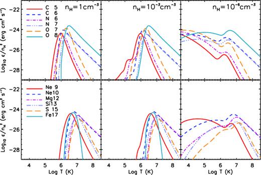
The normalized emissivity, ε/n2H, in units of erg cm3 s−1, of a selection of soft X-ray emission lines as a function of temperature, for constant hydrogen number density and assuming solar abundances in the presence of the redshift z= 0.27 UV/X-ray background. The left, middle and right panels show results for nH= 1, 10−3 and 10−6 cm−3, respectively. If the gas is collisionally ionized, the normalized emissivity is independent of the gas density. Cool diffuse gas is mostly photoionized, while collisional ionization equilibrium dominates for the highest temperatures and densities.
Collisional ionization is the dominant ionization process at the highest densities and temperatures, while the contribution of photo-ionization is largest at low density and at low temperatures. The wings of the emissivity curves at T < 106 K and nH < 10−3 cm−3 are signatures of photo-ionization. The assumption of ionization equilibrium, also used to calculate the cooling tables (Wiersma et al. 2009a), is well justified for photo-ionized regions and dense gas in the centres of clusters (see Bertone et al. 2008 for a review). However, non-equilibrium processes may become important in the WHIM and in the outer regions of groups and clusters (Yoshida et al. 2005; Yoshikawa & Sasaki 2006; Cen & Fang 2006; Gnat & Sternberg 2007). Gnat & Sternberg (2009), in particular, have recently shown that non-equilibrium processes affect the cooling of shock-heated gas with temperatures with 104 < T < 107 K, and that the amplitude of the deviations from ionization equilibrium increases with the gas metallicity. On the other hand, Yoshikawa & Sasaki (2006) found the effect of non-equilibrium ionization to be small for the subject of this paper: metal-line emission from the WHIM.
The emissivities shown in Fig. 1 are comparable to those of Yoshikawa et al. (2003) and Fang et al. (2005), with the exception of the Fe xvii line, which is significantly weaker than found by Fang et al. (2005). In general, we find that cloudy predicts an Fe xvii emissivity a factor of about 2 smaller than the Raymond–Smith code (Raymond & Smith 1977) used by Fang et al. (2005). Part of the reason for this discrepancy could be that two of the five strongest Fe xvii emission lines are missing from the cloudy line list, namely λ 15.01Å and λ 17.10Å. This might be an issue for the cooling of metal-rich gas at T∼ 107 K, where the Fe xvii line can contribute up to 30 per cent of the total cooling rate. On the other hand, this lack of iron lines might be balanced by the high iron abundance assumed in cloudy, compared to that estimated by Lodders (2003).
2.2 Line emission calculations
We investigate the WHIM emission in the soft X-ray band by creating synthetic maps of the surface brightness of individual emission lines. We only include emission from gas with densities nH < 0.1 cm−3, because our simulations lack the resolution and the physics to model the emission from higher density gas, which is expected to be multiphase (see the discussion in Dalla Vecchia & Schaye 2008).
3 EMISSION MAPS
In this section, we present emission maps for the strongest soft X-ray emission lines we have identified as WHIM tracers. All PDFs are calculated using the full simulation box with size 100 h−1 Mpc. However, for clarity we show emission maps for only a fraction of the full box. In particular, we focus on a smaller area of 14 h−1 Mpc on a side that contains one of the largest groups in the simulation, with a total mass of about 7 × 10¹⁴ M☉, a smaller group and a few dense filaments. This choice is motivated by the fact that the strongest emission comes from high-density regions such as groups and filaments.
To illustrate the morphology of the emission, Fig. 2 shows the O viii emission from a slice of the full simulation box in the left-hand panel and two consecutive zooms into the core of a massive group in the companion panels. The displayed regions decrease in size by factors of 10, ranging from 100 h−1 Mpc to 1 h−1 Mpc. The strongest O viii emission is concentrated in the high-density knots at the intersections of filaments, where groups reside, while the emission from cooler and more diffuse gas in filaments and voids is several orders of magnitude weaker. For comparison, the intensity of the unresolved X-ray background is ∼10−2 photon s−1 cm−2 sr−1 (Hickox & Markevitch 2006, see also Section 8) and roughly corresponds to orange in the colour scale. As we will see in the following, the surface brightness of the WHIM is higher than the background only in relatively overdense regions.
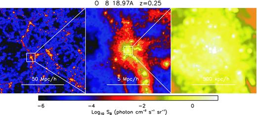
Zoom into an O viii 18.97 Å emission map of a high-density region at z= 0.25. The object at the centre of the displayed region is one of the largest haloes in the simulation, with a total mass of a few times 1014 M☉. The slice thickness is 20 h−1 comoving Mpc (which corresponds to 1772 km s−1). From left-to-right, the pixel sizes are 100, 10 and 1 arcsec and the angular sizes of the regions shown are 8°, 48′ and 4.8′ (corresponding to 100, 10 and 1 h−1 comoving Mpc), respectively. The blobs in the right-hand panel are resolved substructures.
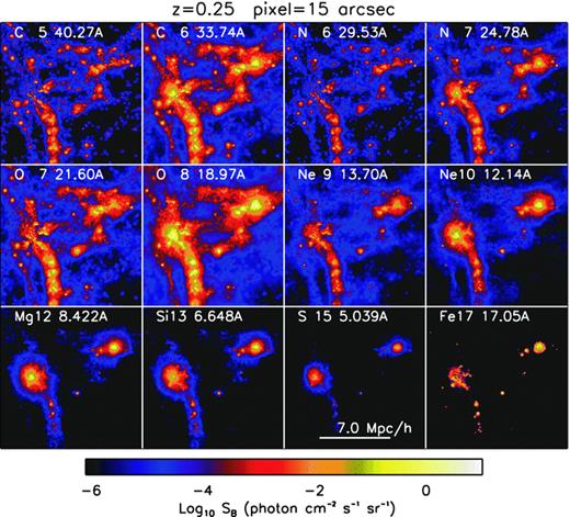
Maps of the emission for a sample of 12 different soft X-ray lines, listed in Table 1, at z= 0.25. The figure shows a zoom of a region, with a comoving size of 14 h−1 Mpc ( on the sky) that includes the largest group in the simulation. The density, temperature and metallicity in this region are shown in Fig. 15. All panels assume the same angular resolution (15 arcsec, which corresponds to a physical size of 42 h−1 kpc) and slice thickness (20 h−1 comoving Mpc, which corresponds to 1772 km s−1). The maximum of the colour scale has been set to a fraction of the real maximum to enhance the emission of the weaker lines and of low-density regions. The O viii line is the strongest emission line in the sample. Carbon, nitrogen, oxygen and neon lines best trace the distribution of the WHIM in filaments and in the outskirts of groups, while lines from elements with higher atomic numbers such as Mg xii, Si xiii, S xv and Fe xvii mostly trace hot and dense gas in massive haloes.
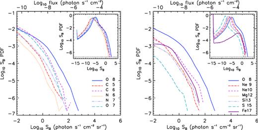
The flux PDFs of the sample of soft X-ray emission lines that are also shown in Fig. 3 and that are listed in Table 1, at z= 0.25. The left-hand panel shows results for C v, C vi, N vi, N vii, O vii and O viii, and the right-hand panel for Ne ix, Ne x, Mg xii, Si xiii, S xv and Fe xvii. The main plotting area shows only the high flux tail of the distributions, while the full PDFs are shown in the inset. The pixel size is 15 arcsec (which corresponds to a physical size of 42 h−1 kpc) and PDFs are calculated using five slices through the simulation box that are each 20 h−1 comoving Mpc thick (which corresponds to 1772 km s−1). In Appendix A3 we show that for sufficiently large fluxes (>10−5 photon s−1 cm−2 sr−1 for O viii) the PDF is proportional to the slice thickness. The O viii line is the strongest emission line in the sample, followed by C vi and Ne x. The Fe xvii can reach high fluxes, but only in a limited number of pixels compared with other lines (see the inset of the right panel). This is due to the different spatial distribution of iron in the IGM and to the sharply declining values of the Fe xvii emissivity curve outside a narrow range around its peak temperature. The intensity of the unresolved X-ray background (∼10−2 photon s−1 cm−2 sr−1, discussed in Section 8) corresponds to the minimum value shown on the x-axis.
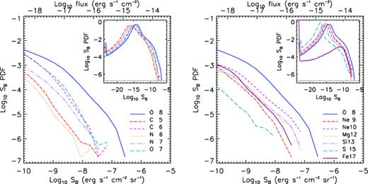
As Fig. 4, but with the emission line flux expressed in erg s−1 cm−2 sr−1, instead of photon s−1 cm−2 sr−1. The relative strength of the lines varies slightly when converted to these units and is more easily comparable to the flux limits proposed for future missions such as IXO and EDGE.
Here, we consider only the strongest lines from hydrogen-like atoms and the resonance lines in triplets from helium-like atoms, and we defer the discussion of the behaviour of lines within the triplet to Section 3.1. These lines have been chosen on the basis of their strength and detectability in the soft X-ray band, but are by no means the only important lines. Although we only show results for one iron line from the Fe xvii ion, we note that the soft X-ray band is a very rich band for iron lines from a multiplicity of other higher-order ions, including, e.g. Fe xviii and Fe xx. Most lines from these ions trace slightly hotter gas than the Fe xvii lines, but nevertheless represent an extremely important cooling channel for hot gas in dense environments. Lines from Fe xvi are instead emitted at longer wavelengths and fall outside the soft X-ray band.
Figs 3, 4 and 5 clearly indicate that O viii λ 18.97Å is the strongest emission line and that for all lines the strongest fluxes are concentrated in very small regions or, equivalently, in a small fraction of the pixels in the maps. All lines are weaker than O viii by a factor of a few or more. This is a consequence of the O viii λ 18.97Å line emissivity, which is highest of all lines, and of the high relative abundance of oxygen. The emissivity of O viii peaks at a temperature T∼ 3 × 10⁶ K, and remains higher than for any other line at higher temperatures. The line emissivities shown in Fig. 1 give a good indication of what lines dominate the emission. However, the total emission in each line is not only determined by the emissivity itself, but also by the fraction of the gas mass and metallicity in the temperature–density plane that corresponds to each emissivity value.
Fig. 3 illustrates how some lines, namely C v, C vi, O vii and Ne ix, preferentially trace the cooler gas in filaments and in the outskirts of groups, while others, namely Ne x, Mg xii, Si xiii and S xv, better trace the hot medium at the centres of groups. This is a direct consequence of the fact that the peak of the emissivity shifts to higher temperatures with increasing atomic number and ionization state, as can be seen in Fig. 1. The C v, O vii and Ne ix lines, whose emissivities peak at about 106 K, 2 × 10⁶ K and 4 × 10⁶ K, respectively, are best-suited to investigate the diffuse gas in filaments and in the outskirts of groups. However, their emission declines drastically in the centres of large haloes, where the gas is very hot and more highly ionized atoms dominate (see e.g. the centres of the groups shown in Fig. 3). Emission lines such as C vi, O viii, Ne x, Mg xii, Si xiii and S xv are the best probes of the dense gas in groups and clusters, but do not trace the low-density gas in filaments and the field as well as C v, O vii and Ne ix do, because their emissivities peak at higher temperatures.
The Fe xvii line is an exception to this trend because, even though its emissivity peaks at T∼ 6 × 10⁶ K, its value is only high in a narrow temperature range. In addition, the spatial abundance of iron differs significantly from that of other elements because of the delay in the SN Ia enrichment. While iron is abundant in the intragroup medium and in the vicinity of galaxies, it is significantly underabundant in the diffuse IGM. The flux PDFs in Fig. 4 show that most lines produce fluxes higher than about 1 photon s−1 cm−2 sr−1 in at least a few pixels.
Fig. 6 shows the relative intensity of lines with respect to each other. When the contours lie above the dashed diagonal line, the emission line on the y-axis produces the highest flux, when below, the line on the x-axis is the strongest. In general, the O viii and C vi lines produce the highest fluxes, both among the lines that trace the hottest gas and among those that trace cooler gas. Lines from helium-like atoms produce higher fluxes than O viii and C vi in a relatively small number of pixels. These correspond to regions of the IGM with relatively low temperatures, where helium-like atoms are the dominant species. The lines in Fig. 6 are sorted by atomic mass and then by ionization state, which is nearly the same as sorting by the temperature for which the emissivity peaks (see Fig. 1). This explains why the contours are much narrower for panels near the diagonal running from the bottom-left to the top-right of the figure than they are for panels near the top-left and bottom-right of the plot: panels near the diagonal correlate lines for which the emissivity peaks at similar temperatures. Fig. 6 illustrates the distribution of line ratios that can be expected in surveys of WHIM emission and may help to confirm the validity of line identifications.
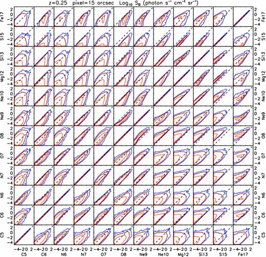
Comparison of the intensities of the lines listed in Table 1. The contours show the number density of pixels and are logarithmically spaced by 1.7 dex. The distributions have been calculated using five 20 h−1 comoving Mpc slices through the simulation box at z= 0.25, assuming an angular resolution of 15 arcsec. Both axes show the line surface brightness Log10SB in units of photon s−1 cm−2 sr−1. The dashed diagonal line in each panel indicates equal fluxes. The O viii and C vi lines produce the highest fluxes. Lines emissivities of which peak at similar temperatures (i.e. panels near the diagonal running from the bottom-left to the top-right of the plot) are strongly correlated.
Although the actual difference in flux between emission lines can be as high as an order of magnitude, all emission lines in our set might be detectable in the centres of galaxy groups and in the outskirts of clusters.
3.1 The O vii triplet
In this section we discuss the properties of line triplets from Helium-like atoms, focussing in particular on the O vii triplet (see Table 1), which should be the easiest to detect. The properties of the lines in triplets are important because the column density of a gas can be estimated using the ratio of the intensity of the resonance line of helium-like atoms and other lines in the triplet. This might be possible, for example, when at least two out of the three lines are detected.
The lines in the triplet correspond to the atomic transition 1s2p→ 1s2 and in particular:4
resonance line: 1P1→1S0
intercombination line: 3P2,3→1S0
forbidden line: 3S1→1S0.
Of the three main emission lines of helium-like atoms, the resonance line is usually of comparable strength to the forbidden line at high density, while the intercombination line is usually the weakest. The forbidden line, however, becomes the dominant emission line in low-density environments, where gas is mostly photo-ionized and radiative intercombination is the dominant line emission process.
Photons at the wavelength of the resonance line can be resonantly scattered in random directions when passing through an intervening medium, while photons at the intercombination and forbidden frequencies have negligible cross-sections. As such, only the intensity of the resonance line can be attenuated along the line of sight, giving rise to absorption in the spectra of background objects. Interestingly, as Churazov et al. (2001) point out, the photons of the cosmic X-ray background are scattered in the same way, therefore boosting the line emission of the WHIM gas in filaments where the scattering occurs, compared to the thermal emission from the gas itself. This effect might improve the chances of detecting the WHIM in emission (Yoshikawa et al. 2003).
In Fig. 7, we show the flux predicted for the resonance, intercombination and forbidden lines in the O vii triplet. The flux PDF of the same lines is shown in Fig. 8, while Fig. 9 compares the flux intensity of pairs of lines on a pixel-by-pixel basis. The intensity of the intercombination line is about two to 10 times smaller than those of the forbidden and resonant lines. At the highest fluxes, F≥ 10−3 photon s−1 cm−2 sr−1, corresponding to high-density regions, as we will show in the following sections, the intensity of the resonance line matches that of the forbidden line well, and the shapes of the PDFs are basically the same. At lower densities, the fluxes predicted for the forbidden line become higher than those of the resonance line by up to a factor of 10. This can be seen, for example, as a blue glow in voids in the right-hand panel of Fig. 7, while the flux of the resonance line in the left-hand panel is lower than the minimum of the colour scale. As a consequence, the ratio of the intensity of the resonance and the intercombination line, as well as the ratio of the resonance and the forbidden line, varies (left and middle panels of Fig. 9), while only the ratio of the intercombination and forbidden lines is constant (right-hand panel of Fig. 9).
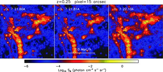
As Fig. 3, but comparing the resonance (left-hand panel), intercombination (middle panel) and forbidden (right-hand panel) emission lines of the O vii triplet. The resonance and forbidden lines have similar strengths in dense regions with strong emission, but the forbidden line becomes the main emission channel in lower density regions with fluxes lower than about 10−3 photon s−1 cm−2 sr−1.
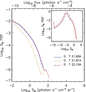
As Fig. 4, but for the flux PDFs of the O vii triplet emission lines. The fluxes from the resonance and forbidden lines are about equal for Log10F > −3 photon s−1 cm−2 sr−1, but at lower fluxes the forbidden line becomes the dominant emission channel, while the intercombination line becomes as strong as the resonance line.
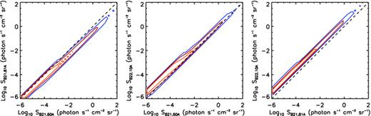
As Fig. 6, but for the line intensities in the O vii triplet: intercombination line versus resonance (left-hand panel), forbidden versus resonance (middle panel) and forbidden versus intercombination (right-hand panel).
In the absence of absorption by an intervening medium, both the forbidden and the resonance lines might be used to investigate the properties of WHIM gas. However, in low-density regions such as filaments and in the presence of an optically thick layer of gas, the forbidden line might be a better tracer of the WHIM. On the other hand, the resonance line is the only useful line for comparisons with absorption studies, such as those planned for IXO.
4 ANGULAR RESOLUTION
In this section, we investigate the effect of varying the angular resolution of the detector.
Fig. 10 compares the PDFs of the measured flux of O viii emission assuming angular resolutions of ϑ= 5 arcsec, 15 arcsec, 1 arcmin, 4 arcmin and 10 arcmin. The distributions roughly converge for low fluxes, but there is no convergence at the highest fluxes and reducing the pixel size continues to increase the highest observed flux, at least down to the smallest scale considered here. This is because larger pixel sizes prevent the detection of very strong emission coming from structures with an angular size smaller than that used to observe them. When observing diffuse gas on scales larger than galactic scales (such as the WHIM), an angular resolution of about 10–15 arcsec is sufficient at z∼ 0.25 and does not imply a significant loss of information. However, higher angular resolution might be desirable when observing gas with more clumpy spatial distribution on smaller scales, such as outflowing gas in galactic winds. For reference, in the OWLS cosmology a pixel size of 15 arcsec subtends a comoving (proper) size of about 52 (42) h−1 kpc at z= 0.25, 98 (66) h−1 kpc at z= 0.5 and 175 (87) h−1 kpc at z= 1.
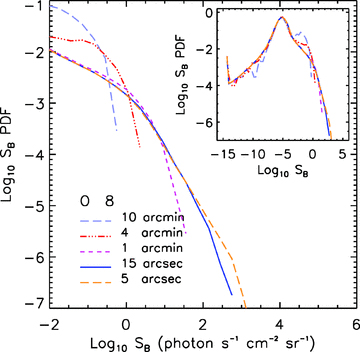
As Fig. 4, but for O viii emission as a function of the angular resolution of the emission maps. The pixel sizes are ϑ= 5 arcsec, 15 arcsec, 1 arcmin, 4 arcmin and 10 arcmin, corresponding to physical sizes of 14 h−1 kpc, 42 h−1 kpc, 166 h−1 kpc, 665 h−1 kpc and 1.661 h−1 Mpc, respectively. Results broadly converge at high angular resolution (ϑ≲ 1 arcmin), except for the highest fluxes at the centres of haloes, which arise from gas in clouds with physical dimensions smaller than the pixel sizes considered here. There is no clear convergence at low angular resolutions (ϑ > 1 arcmin).
5 EVOLUTION
In this section, we briefly discuss how the intensity of the emitted flux varies with cosmic time.
As mentioned in the previous section, as redshift increases, the physical size that corresponds to a pixel of a constant angular size increases steadily, at least up to z= 1. Moreover, the intrinsic emission depends on the temperature, density and metallicity of the gas itself, as well as on the UV/X-ray background, all of which evolve. In Fig. 11, we show the flux PDF of O viii emission at redshifts z= 0.25, 0.5 and 1. The overall shape of the flux PDF changes little with redshift, but the change is most noticeable at the highest fluxes, where the maximum flux decreases with increasing redshift. This is at least partly due to the fact that at constant angular resolution and over the redshift range considered here, pixels correspond to larger physical sizes at increasing redshifts and, as shown in Section 4, the maximum flux decreases with increasing pixel size.
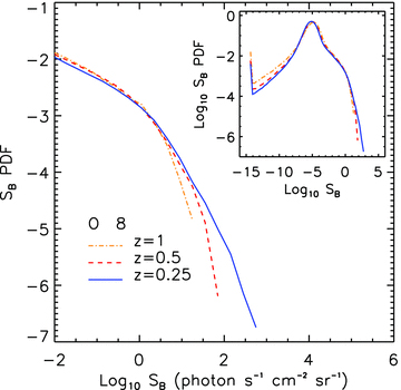
As Fig. 4, but for O viii emission as a function of redshift. Results are shown at z= 0.25, 0.5 and 1. Maps are created assuming constant angular resolution ϑ= 15 arcsec, which implies the physical size of a pixel increases with redshift from 42 h−1 kpc at z= 0.25 to 88 h−1 kpc at z= 1. The flux PDFs are nearly the same, but diverge at the highest fluxes. In particular, the highest fluxes are found at the lowest redshift. This is probably mostly due to the varying physical size of the pixels.
6 WHAT TYPE OF GAS DOMINATES THE EMISSION?
In this section, we investigate what type of gas contributes most of the soft X-ray emission. We begin by showing the emission-weighted gas distribution in the temperature–density plane for several lines in Section 6.1. In Section 6.2, we then correlate the O viii flux from individual particles with their density, temperature and metallicity. Finally, we calculate the O viii emission from gas in different density and temperature ranges in Section 6.3.
6.1 Temperature–density plane
Fig. 12 compares the mass-weighted and the metal mass-weighted temperature–density distributions of gas at z= 0.25. The vertical line at nH= 0.1 cm−3 indicates the density threshold above which star-forming particles are put on a power-law EOS (see Section 2) and the horizontal lines at T= 105 K and T= 107 K delimit the temperature range that defines the WHIM.
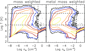
The mass-weighted (left-hand panel) and metal-mass-weighted (right-hand panel) temperature–density distribution of gas at z= 0.25. The large difference between the two distributions implies that the bulk of the metals do not trace the bulk of the gas mass. The contours are logarithmically spaced by 1.5 dex. The horizontal lines at constant temperature highlight the WHIM range, while the vertical line at nH= 0.1 cm−3 indicates the limit above which we impose an EOS on to star-forming particles. These dense particles are excluded from the calculation of the emission. For reference, the cosmic mean density corresponds to nH≈ 3.7 × 10⁻⁷ cm−3.
The mass-weighted and the metal mass-weighted distributions in Fig. 12 clearly indicate that the bulk of the metals do not trace the bulk of the gas mass. A large fraction of the gas mass resides in the low-density IGM with T < 105 K, while metals are more common in the moderately dense WHIM (see also Wiersma et al. 2009b). Also, a significant fraction of metals are found in the relatively dense gas which populates the branch of the distribution with nH > 10−2 cm−3 and T < 105 K. This gas is accreting on to galaxies and may eventually end up in the interstellar medium (ISM).
Fig. 13 presents the emission-weighted temperature–density distributions of the gas, where the weight is given by the emission in a different line in each panel. The lines we consider here are C v, C vi, N vi, N vii, O vii, O viii, Ne ix, Ne x, Mg xii, Si xiii, S xv and Fe xvii, as listed in Table 1. Comparison of the mass-weighted, metal-mass-weighted and the emission-weighted temperature–density distributions demonstrates that neither the bulk of the mass nor the bulk of the metals are good tracers of the bulk of the soft X-ray emission from metal lines. The peak of the emission-weighted distributions of all lines is shifted towards higher densities, compared to the mass- and metal-mass-weighted distributions. In fact, the emission of virtually all highly ionized ions emitting in the X-ray band concentrates in a region of the temperature–density plane with nH > 10−5 cm−3 and T > rsim 106 K. While the emission from hydrogen-like atoms is strong also for temperatures in excess of 107 K, emission from helium-like atoms such as C v, N vi and O vii peaks at T < 107 K and declines steeply at higher temperatures.
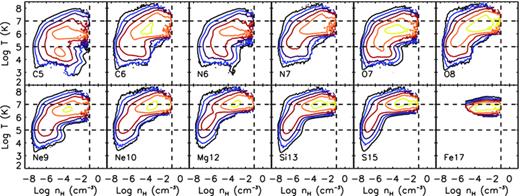
The emission-weighted temperature–density distributions of gas at z= 0.25. The distributions are weighted by the emission in different line for different panels, as indicated in the bottom-left corner of each panel. From left to right and from top to bottom, the lines are: C v, C vi, N vi, N vii, O vii, O viii, Ne ix, Ne x, Mg xii, Si xiii, S xv and Fe xvii. The contours are logarithmically spaced by 1.5 dex and represent equal emission levels in all panels. The horizontal dashed lines at constant temperature highlight the WHIM range, while the vertical line at nH= 0.1 cm−3 indicates the limit above which we impose an effective EOS on to star-forming gas. We do not include emission from this high-density gas. For reference, the cosmic mean density corresponds to nH≈ 3.7 × 10⁻⁷ cm−3. Lines from atoms with low atomic numbers are better tracers of WHIM emission, while lines from heavier elements and from hydrogen-like ions mostly trace hotter gas with temperatures in excess of 107 K. Fe xvii emission is only present in a very narrow temperature range, while C vi and O viii lines trace gas in a wide temperature range.
Fig. 13 demonstrate that, among the ones shown here, the best lines to trace the WHIM in the temperature range 106 K < T < 107 K are C vi, N vi, N vii, O vii, O viii and Ne ix. All other ions tend to trace hotter and somewhat denser gas with T > rsim 107 K and nH > 10−4 cm−3.
6.2 Correlations between luminosity and gas properties
Fig. 13 shows what densities and temperatures dominate the global emissivity in various emission lines, but much of this emission may come out at fluxes that are too faint to be detectable. It is therefore also of interest to investigate physical conditions in the gas that produces the brightest emission.
Fig. 14 quantitatively investigates the dependence of C vi, O vii, O viii and Ne x emission on the gas properties for a sample of emission lines by showing the median values of the particle density (left-hand panel), temperature (middle panel) and metallicity (right-hand panel) that produce a given particle luminosity. Since we consider individual particles for this plot, the density, temperature and metallicity in Fig. 14 are local quantities, and as such cannot be compared directly with those shown in Fig. 15 in the following section and with the average quantities inferred observationally for the ICM and IGM. This is important for the metallicity, as the metal distribution in our simulations is inhomogeneous on small scales. The scatter of the distributions, which is not shown, is relatively small at high fluxes and increases at lower fluxes to up to 0.5 dex.
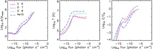
Median values of the gas particles's overdensity (left-hand panel), temperature (middle panel) and metallicity (right-hand panel) that produce a given X-ray particle flux at z= 0.25 for the lines C vi, O vii, O viii and Ne x. Note that fluxes are given in units of photon s−1 cm−2, but that previous figures used photon s−1 cm−2 sr−1. Because we plot the flux emitted per particle, it is directly dependent on the numerical resolution. The absolute normalization of the x therefore does not contain any useful information. For reference, ρmean(z= 0.25) corresponds to nH≈ 4 × 10⁻⁷ cm−3 and our star formation threshold corresponds to log10ρ/ρmean≈ 5.4. Note that emission from higher density gas (i.e. the ISM) was ignored. The median density and metallicity increase with luminosity, while the median temperature flattens out at the peak temperature of the emissivity of each line.
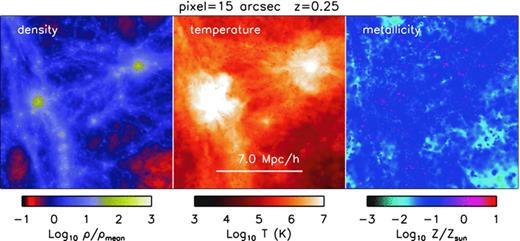
As Fig. 3, but showing maps of the gas overdensity (left-hand panel), temperature (middle panel) and metallicity (right-hand panels).
The trends observed in Fig. 14 are consistent with the results of Fig. 13. The line flux is strongly correlated with density and metallicity, and the highest fluxes are always produced by dense and metal-rich gas near galaxies. These correlations are not surprising, because the emission scales with the element abundance and with the density squared. On the other hand, the median gas temperature that produces a given flux is almost constant at the highest fluxes and quickly decreases at the lowest fluxes. This is a direct consequence of the fact that the line emissivity peaks in a narrow temperature range, as shown in Fig. 1. The specific value of the median temperature at the highest fluxes is almost equivalent to the temperature where the line emissivity peaks, as also seen in Fig. 13. This suggests that the detection of a specific emission line yields the temperature of the gas with a small degree of uncertainty. The value of the observed flux then provides information about the density and the metallicity of the gas. The degeneracy between the two might be hard to break without further data from multiple lines from different elements and ionization states, but it appears from Fig. 14 that, at the bright end, the flux increases faster with the gas density than with the metallicity.
For each line, the maximum flux is reached at the density that corresponds to our star formation threshold. Because we lack both the physics and the resolution to model the gas at higher densities (recall that we impose an effective EOS on to the ISM), we have ignored emission from higher densities. The peak fluxes are therefore limited by this density cut. We stress that this means that the models presented here underestimate the maximum fluxes. On the other hand, the higher fluxes arise in gas with densities typical of the ISM and can therefore hardly be counted as WHIM.
Finally, we note that the trends with density and temperature remain the same if we assume a constant metallicity rather than the metal distribution predicted by the simulation.
6.3 Density and temperature cuts
In this section, we create O viii emission maps using only gas with temperatures and densities in a given interval. This will help us to understand the dependence of the emission on temperature and density, and will give an indication of what type of gas produces what kind of emission. For comparison, we show in Fig. 15 the density, temperature and metallicity of the gas in the same region of space shown in all the emission maps in this paper.
Fig. 16 shows O viii emission maps made using only gas with temperatures in a specific range. We consider the four temperature intervals T < 105 K, 105 K < T < 106 K, 106 K < T < 107 K and T > 107 K. Similarly, in Fig. 17 we consider four different density intervals, with  varying by 1 dex in each density bin. The flux PDFs for the entire simulation volume are shown in Fig. 18 for the temperature cuts and in Fig. 19 for the density cuts. Figs 16–19 demonstrate that the strongest O viii emission comes from gas in dense (
 ) and hot (T > 106 K) regions.
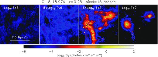
As Fig. 3, but showing maps of O viii emission from gas in four different temperature ranges. From left to right: T < 105 K, 105 K < T < 106 K, 106 K < T < 107 K and T > 107 K. The highest O viii fluxes are produced by gas with T > 106 K. O viii emission is strongest in the highest temperature range.
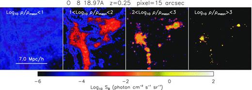
As Fig. 3, but showing maps of O viii emission for gas in four different density ranges, as indicated at the top of each panel. The highest fluxes are associated with the densest gas.
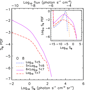
As Fig. 4, but showing the PDF of the O viii flux from gas in different temperature intervals. The highest O viii flux is produced by gas with T > 106 K. O viii emission is weakest in the lowest temperature ranges.
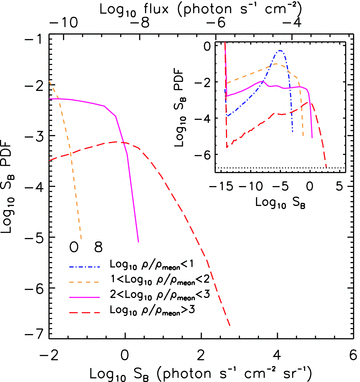
As Fig. 4, but showing the PDF of the O viii flux from gas in different density intervals. The highest fluxes are associated with the densest gas. In particular, the flux predicted for gas outside the virial radii of haloes (i.e. ρ/ρmean≲ 200) is at least a few orders of magnitude weaker than the flux from denser regions.
7 DEPENDENCE ON THE PHYSICAL MODELS
A key feature of the OWLS project is the availability of a large number of runs with varying physical prescriptions. In this section we investigate how a series of physical prescriptions affect the predictions for the WHIM emission. We will only show results for O viii λ 18.97Å emission, but note that we find similar trends for other lines. We focus on a subset of the OWLS models with varying feedback schemes and cooling recipes, which are the physical implementations that produce the largest variations in the diffuse emission. These runs differ not only in the total amount of metals produced and in the spatial distribution of the metals, but also in the star formation history (Schaye et al. 2010) and in the density and temperature distribution of the diffuse gas. Physical prescriptions are changed one at a time in order to isolate their impact on the results. The physical models considered here are the following [we refer the reader to Schaye et al. (2010) and to the works cited below for more detailed descriptions]:
REF: Our reference model, as described in Section 2. All results presented in the preceding sections were obtained from this simulation. This model uses the star formation prescription of Schaye & Dalla Vecchia (2008), the supernova-driven wind model of Dalla Vecchia & Schaye (2008) with wind mass loading η= 2 and wind initial velocity vw= 600 km s−1, the metal-dependent cooling rates of Wiersma et al. (2009a), the chemical evolution model described in Wiersma et al. (2009b) and the WMAP3 cosmology. AGN feedback is not included.
NOSN: As REF, but without supernova feedback. The metals produced by stars are only transported by gas mixing and no energy is transferred to the IGM and ISM when SNe explode.
NOZCOOL: As REF, but with radiative cooling rates calculated assuming primordial abundances. The neglect of the contributions of metal lines implies slower gas cooling than in the REF model.
AGN: As REF, but with the addition of AGN feedback as described in Booth & Schaye (2009).
WML4: As REF, but with a wind mass loading twice as high, that is η= 4. The total energy injected in winds is thus also twice that in REF.
- WDENS: As REF, but the wind properties scale with the local gas density as (Schaye et al. 2010)5
 where ρcrit is the density threshold for star formation, vw0= 600 km s−1 and η0= 2. This implies that at ρcrit the gas is kicked with the same velocity and mass loading as in the REF model. This particular scaling of wind velocity with density was chosen so that the wind velocity scales with the local sound speed (recall that we impose the EOS P∝ρ4/3 on to the ISM) and the wind mass loading is scaled such that the total wind energy is independent of the gas density. As a consequence, the wind energy is equal to that in the REF model.6
WVCIRC: As REF, but with ‘momentum-driven’ galactic winds following the prescription of Oppenheimer & Davé (2008), with the difference that winds are ‘local’ to the star formation event and are fully hydrodynamically coupled as in the REF model (see Dalla Vecchia & Schaye 2008 for a discussion of the importance of these effects). The wind initial velocity and the wind mass loading factor are defined as a function of the galaxy velocity dispersion σ as vw= 5σ and η=vw0/σ, respectively, with vw0= 150 km s−1. The velocity dispersion
 is estimated using an on-the-fly friends-of-friends halo finder. This model was motivated by the idea that galactic winds may be driven by radiation pressure on dust grains rather than supernovae. The energy injected into the wind becomes much higher than for REF for halo masses exceeding 1011–1012 M☉.
MILL: As REF, but using the WMAP year 1 cosmology (Spergel et al. 2003) as in the Millennium simulation (Springel et al. 2005) and a wind mass loading factor η= 4. Results from this model must be compared to those of the WML4 model to isolate the effect of cosmology.
DBLIMF: As REF, but using a top-heavy IMF at high gas pressures. This model switches from a Chabrier IMF to a power-law IMF dN/ dM∝M−1 (as compared to ∝M−2.3 for the high-mass tail of the Chabrier IMF) at the critical pressure P/k= 2.0 × 106 cm−3 K, which was chosen because for this value ∼10−1 of the stellar mass forms at higher pressures. The extra SN energy is used to increase the initial wind velocity to 1618 km s−1 for star particles formed with a top-heavy IMF, while keeping the mass loading factor fixed at η= 2 (as for the Chabrier IMF, these parameter values correspond to 40 per cent of the available SN energy). This model is called DBLIMFCONTSFV1618 in the OWLS project (which includes more models with top-heavy IMFs in starbursts; see Schaye et al. 2010).
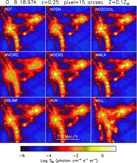
Fig. 20 shows maps of the O viii emission for all runs in a region of 14 h−1 Mpc on a side or, equivalently,  on the sky. Fig. 21 shows the emission in the same simulations, but for a constant gas metallicity of Z= 0.1 Z☉. Figs 22 and 23 present the flux PDFs of the O viii emission using the predicted abundances and Z= 0.1 Z☉, respectively.
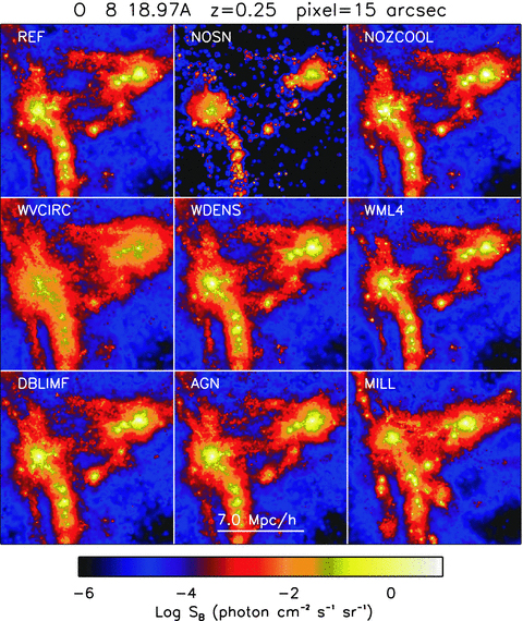
As Fig. 3, but showing O viii emission maps for different simulations, as indicated in the top left corner of each panel.
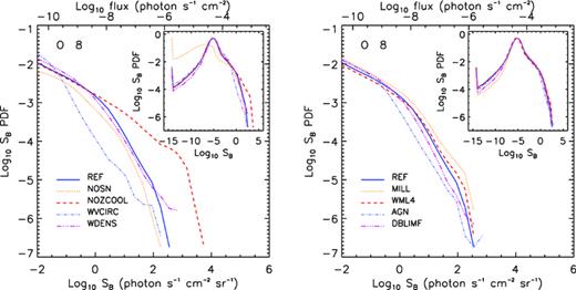
As Fig. 4, but showing the flux PDFs of O viii emission for simulations with varying physical prescriptions. The simulations shown in the left-hand panel are the same ones as in Fig. 20. Additional runs are shown in the right-hand panel and compared to the results of the REF run. The results are surprisingly robust to changes in the physical model. However, neglecting metal-line cooling results in a large overestimate of the maximum flux. Ignoring supernova-driven winds has little effect for the brightest pixels, but otherwise shifts the PDF to lower fluxes.
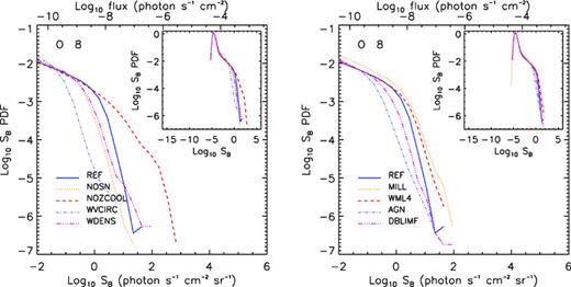
As Fig. 4, but showing the flux PDFs of O viii emission for simulations with varying physical prescriptions, under the assumption of a constant gas metallicity of Z= 0.1 Z☉. The simulations shown are the same ones as in Fig. 20. The assumption of constant metallicity boosts the flux from the low-density, cool regions of the universe, where the largest contribution to the line emissivity comes from photo-ionization by the UV background (compare the inset to that of Fig. 22), but it reduces the maximum fluxes. The differences between the models are qualitatively the same as when the predicted metal distributions are used (compare with Fig. 22).
The dominant impression we get from looking at these figures is that most models predict very similar O viii fluxes. This is somewhat surprising, as the physics that is included is quite different and the models predict a rather wide range of star formation histories (Schaye et al. 2010). Closer inspection does, however, reveal several differences. Visually, we can easily see from the top panels of Fig. 20 that models NOSN, WVCIRC and MILL differ most from our reference model. Comparing Figs 20 and 21, we see that for NOSN the difference is driven by the metal distribution. Without galactic winds, the metals remain mostly confined to the inner parts of haloes and the flux from low-density gas is sharply reduced. The predicted metal distributions can, however, not account for the differences seen for WVCIRC and MILL. The flux from high-density gas is considerably lower for WVCIRC, which indicates that the peak densities are lower and/or that the temperatures of high-density gas are lower than the value for which the emissivity of O viii peaks (i.e. 106.3 K). The MILL run appears different mostly because structure formation has progressed further in this run, because it uses a higher value of σ8.
The flux PDFs shown in Figs 22 and 23 confirm the conclusions drawn from the visual inspection of the emission maps. Looking first at the global distributions shown in the insets, we see that only NOSN differs substantially, the peak of the PDF having shifted to much lower fluxes. If a constant metallicity is assumed, then all models agree near the peak of the distribution and the low-flux tail of the PDF vanishes. This indicates that fluxes ≪10−5 photon s−1 cm−2 sr−1 imply gas metallicities ≪0.1 Z☉. For all models the peak fluxes are lower if a constant metallicity is assumed, from which we conclude that the high flux tail probes gas with metallicities in excess of 0.1 Z☉.
The model for which the high-flux tail differs the most is NOZCOOL, which neglects metal-line cooling. Its flux PDF starts to differ from that of REF for fluxes ≳1 photon s−1 cm−2 sr−1, reaching a maximum flux that is about an order of magnitude higher. The fact that metal-line cooling is important is not surprising, as the metal-line emission that we are studying dominates the radiative cooling rates for temperatures typical of the WHIM and for metallicities >rsim10−1 Z☉ (e.g. Wiersma et al. 2009a). Ignoring metal-line cooling during the simulations leaves the gas in the temperature–density regime where it emits efficiently, artificially boosting the predicted fluxes. The calculation of the emission from metals in this model is, of course, inconsistent with the assumption of primordial abundances used to calculate the gas cooling rates. However, this inconsistency is present in other work (e.g. Fang et al. 2005), which often used cooling rates based on primordial abundances during the simulations and calculates the metal-line emission of the gas in post-processing. Clearly, this approach will strongly overestimate the maximum fluxes.
While the emission map of the MILL model appeared to be substantially different (Fig. 20), the change in cosmology does not change the statistics of the O viii emission substantially, as can be seen by comparing the flux PDFs of the WML4 and MILL models.
There are enormous differences in the feedback processes that are included in the simulations shown here, ranging from no galactic winds (NOSN), to efficient winds driven by supernovae (WDENS), to extremely strong winds in starbursts resulting from a top-heavy IMF (DBLIMF), to violent AGN feedback (AGN). These differences strongly affect the star formation histories (Schaye et al. 2010), yet the flux PDFs of all these models are strikingly similar. This suggests that the metal distributions are also similar in the gas that emits O viii efficiently. Indeed, we will show elsewhere (McCarthy et al. 2010; Wiersma et al. 2010) that the metallicity of the WHIM (much more so than that of other components) is remarkably robust to changes in the feedback prescription. Indeed, assuming a constant metallicity does not change the relative difference between the models much. This suggests that the differences in the high flux tails are driven by differences in the distribution of the baryons in the temperature (T∼ 106.5 K) and density (ρ≫ 103ρmean) regime that dominates the emission from the brightest regions (see Fig. 14). In particular, it appears that the ‘momentum-driven’ winds (WVCIRC), which predict substantially lower peak fluxes (even for a constant metallicity), substantially reduce the peak gas densities of the WHIM. This suggests that these winds are able to remove more gas from the centres of haloes, perhaps because the winds in this model use much more energy than is available from supernovae.
Thus, we conclude that bright O viii emission, and other soft X-ray lines too, may tell us more about the gas densities in the centres of haloes than about the metallicities and the temperatures (which must be close to the peak of the emissivity curve for the emission to be bright). This is because the emissivity scales as Zρ2 and is thus most sensitive to the gas density.
8 CAN THE WHIM BE DETECTED IN EMISSION?
In this section, we discuss the possibility that current and future X-ray telescopes may detect the WHIM emission at the levels predicted by our simulations.
Previous studies predict that X-ray emission from the WHIM is far below the detection threshold of the Chandra and XMM–Newton telescopes (Yoshikawa et al. 2003, 2004; Fang et al. 2005). Predictions that WHIM emission lines in filaments could be detected by XMM–Newton have not been confirmed (Pierre et al. 2000). However, future missions, such as EDGE (Piro et al. 2009), IXO and Generation-X (Windhorst et al. 2006), have been shown to have a better chance of detecting diffuse emission (Yoshikawa et al. 2004; Fang et al. 2005; Bregman 2007).
Ideally, the emission from the WHIM requires an instrument which couples a large FOV with high angular and spectral resolution (Yoshikawa et al. 2004; Fang et al. 2005; Paerels et al. 2008). While instruments with high angular and spectral resolutions alone are fine for searches of absorption features, a large FOV is desirable for mapping diffuse emission. High angular resolution is also very important, as we found that the emission is dominated by bright, compact regions. Without sufficient angular resolution, it will not only be more difficult to detect the emission, but one would also risk misinterpreting its origin. For example, emission that looks smooth and filamentary at poor angular resolution may come from unresolved, dense knots rather than from diffuse, low-density gas.
A few dedicated small to medium sized missions have been proposed to investigate the WHIM emission. The Missing Baryon Explorer (MBE; Fang et al. 2005) was the first of such medium-sized missions, later followed by the Diffuse Intergalactic Oxygen Surveyor (DIOS; Ohashi et al. 2006), the Extreme phySics in the TRansient and Evolving cosMOs (ESTREMO; Piro et al. 2006), EDGE (Piro et al. 2009) and Xenia (Hartmann et al. 2009). The last two missions are very similar. The common goal of all these missions is to build an instrument with a large FOV and high spatial and spectral resolution.
The proposed technical specifications of the instruments we consider are listed in Table 3. The FOV of the X-ray Microcalorimeter Spectrometer5 (XMS) on board IXO is 5.4 × 5.4 arcmin2, which corresponds to 1.1 h−1 comoving Mpc at z= 0.25. Also on IXO, the Wide Field Imager (WFI; Treis et al. 2009) has a FOV of 18 × 18 arcmin2, corresponding to 3.7 h−1 comoving Mpc at the same redshift. Both instruments have sufficient coverage to image gas in filaments at z∼ 0.25, with an angular resolution of 5 arcsec each. For comparison, the WFI and the Wide Field Spectrometer (WFS) on Xenia were proposed to have FOVs of 1° and  and angular resolutions of 15 arcsec and 3.7 arcmin, respectively. While XMS on IXO and WFS on Xenia have impressive energy resolutions of about 3 eV, it is much worse for the WFIs (150 eV for IXO and 70 eV for Xenia).
Summary of the technical characteristics of the instruments on IXO and Xenia.
| Instrument | Effective area (m2) | FOV (arcmin2) | Angular resolution (arcsec) | Energy range (keV) | Energy resolution (eV) |
| IXO | |||||
| XMS | 3 @1.25 keV | 5.4 × 5.4 | 5 | 0.3–7.0 | 2.5 @central 2 × 2 arcmin2 |
| WFI | 3 @1.25 keV | 18 × 18 | 5 | 0.1–15 | 150 |
| Xenia | |||||
| WFS | 0.12 @0.6 keV | 42 × 42 | 222 | 0.1–2.2 | 3 @0.5 keV |
| WFI | 0.058 @1 keV | 60 × 60 | 15 | 0.3–6 | 70 @1 keV |
The unresolved cosmic X-ray background has been measured to be ≈13 ± 1 photon s−1 cm−2 sr−1 keV−1 in the range 0.5–1 keV (Hickox & Markevitch 2006) and is thought to be dominated by diffuse Galactic and local thermal-like emission. For the energy resolution of the XMS (ΔE= 2.5 eV), this corresponds to about 3 × 10⁻² photon s−1 cm−2 sr−1.
The instrumental background for XMS is about 2 × 10⁻² photon s−1 keV−1 per cm−2 of the detector area (Kaastra, private communication). For a pixel size of 300 μm and 3 arcsec, this corresponds to 8.5 × 10¹¹ photon s−1 sr−1 keV−1. For an effective area of 2 × 104 cm2 and an energy resolution of 2.5 eV, this implies a limiting surface brightness of 1.1 × 10⁻² photon s−1 cm−2 sr−1, slightly below the extragalactic background. Thus, we expect observations to become background limited below 10−1 photon s−1 cm−2 sr−1. For an angular resolution of 15 arcsec and an effective area of 2 × 104 cm2, this surface brightness would result in about 10 detected photons per resolution element in a 1 Ms exposure. Hence, with an instrument like XMS it would be possible to detect surface brightnesses ≳1 photon s−1 cm−2 sr−1 (at 15 arcsec resolution) with high confidence in reasonable exposure times. Fig. 19 shows that this would enable the detection of O viii from gas with ρ > rsim 102ρmean at z= 0.25.
For the proposed WFS for Xenia, the instrumental background is expected to be even lower and the energy resolution similar to that for XMS on IXO. The angular resolution is, however, much poorer (about 4 arcmin) and the effective area is an order of magnitude smaller (103 cm2). A 1 Ms exposure would in that case yield ∼102 photons per resolution element for a surface brightness of 10−1 photon s−1 cm−2 sr−1, more than sufficient for a robust detection. Note that XMS on IXO would detect an order of magnitude more photons when averaged over the same angular size (because its effective area is an order of magnitude larger). We predict from the equivalent version of Fig. 19 for a pixel size of 4 arcmin (not shown) that this surface brightness limit is sufficient to detect some O viii emission from gas with ρ > 103ρmean at z= 0.25. Note that while this emission would appear to be diffuse due to the low angular resolution, it would in fact come from unresolved, dense clouds.
Compared with the WFS, the WFI for Xenia has much better angular resolution (15 arcsec), a smaller effective area (about 0.6 × 103 cm2) and a much worse energy resolution (ΔE= 70 eV). Because the spectral resolution is more than an order of magnitude lower than for the WFS, the backgrounds will be higher by the same factor. For reasonable exposure times (∼1 Ms), we would still not be background limited. The poor spectral resolution would, however, make it much more challenging to interpret the observations, as the lines correspond to the differential Hubble flow across a comoving distance ∼250 h−1 Mpc (for z= 0.25). On the other hand, the interpretation would be greatly facilitated by the much improved angular resolution, although this will not necessarily help with the identification of the lines.
The WFI for IXO has an energy resolution that is lower still, ΔE= 150 eV, which may lead to severe projection effects and which would make it challenging to identify the lines. While WFI does not have a better angular resolution than XMS, it does have a much larger FOV (18 arcmin versus 2 arcmin for the high energy resolution mode of XMS).
According to our predictions, the WFS on Xenia should be able to detect strong emission from the WHIM only for gas with overdensities greater than 1000, such as in the centres of groups IXO would be extremely exciting as it would be sufficiently sensitive to detect emission from O viii, and probably a few other lines, from both the cores of small groups and the outskirts of larger groups and clusters down to overdensities >rsim102, and with an angular resolution that is sufficient to resolve much of the intrinsic structure.
Instruments with higher sensitivity and lower flux limits will be required in the future to image the emission from the diffuse WHIM in low-density regions and in filaments where ρ≪ 102ρmean. Generation-X (Windhorst et al. 2006) might be one of those missions. Since most of the baryons contained in the WHIM reside at such low overdensities (Fig. 12), it seems unlikely that the bulk of the baryons will be detected in soft X-ray emission any time soon. Absorption experiments clearly have a better chance to accomplish this goal.
However, we have seen that detecting soft X-ray emission from the gas in and around (groups of) galaxies is within reach of proposed missions. This is extremely exciting, as such observations would provide vital clues on gas infall, outflows and metal enrichment, which are the key, poorly understood processes in models of the formation of galaxies.
9 CONCLUSIONS
Gravitational accretion shocks and, to a lesser extent, galactic winds driven by supernovae and/or AGN, can shock-heat the diffuse IGM to temperatures >rsim105 K. At low redshifts, a large fraction of the baryons are thought to reside in this WHIM (105< T < 107 K) and soft X-ray emission lines from metals offer a way to detect them.
Here, we used a subset of cosmological simulations from the OWLS project (Schaye et al. 2010) to study the nature and detectability of this emission. These simulations are among the largest dissipative runs ever performed, and use new prescriptions for a range of baryonic processes, such as star formation, galactic winds driven by massive stars and supernovae, and feedback from AGN. Of particular relevance for us is that they are fully chemodynamical, tracking the delayed release of 11 different elements by massive stars, supernovae of Types II and Ia, and asymptotic giant branch stars, and that radiative cooling is implemented element-by-element in the presence of an evolving UV/X-ray background.
Our main conclusions can be summarized as follows.
The strongest emission in the soft X-ray band comes from the O viii line, whose emissivity peaks at a temperature of a few times 106 K. A large number of other lines are, however, only slightly weaker.
Emission lines from metals provide strong constraints on the temperature of the emitting gas. Most of the emitted radiation and essentially all of the potentially detectable flux come from gas with temperatures close to the peak of the emissivity curve for a collisionally ionized gas. Because of the quadratic dependence of the emissivity on density, the emission traces neither the bulk of the baryonic nor the bulk of the metal mass. Instead, the emission is dominated by metal-rich gas at very high overdensities in and around galaxies. Since the peak temperature of the emissivity increases with atomic number and ionization state, lines from heavier or more highly ionized atoms trace hotter gas. As such, C vi and O vii trace gas with T∼ 106 K, O viii, Ne ix and Fe xvii gas with 106 K < T < 107 K, and Ne x, Mg xii, Si xiii and S xv gas with T∼ 107 K.
By comparing results from different OWLS models, we have investigated the dependence of the results on a number of physical mechanisms. It is essential to accurately model the cooling rates. In particular, studies that neglected metal-line cooling are not self-consistent and will have overestimated the maximum fluxes by about an order of magnitude. Without galactic winds, the PDF of the flux shifts to much lower values. However, the high-flux tail, which will become detectable first, is surprisingly robust to strong variations in the strength of the winds, remaining similar even when galactic winds are turned off or when violent AGN feedback is included. While assuming a constant metallicity of 0.1 Z☉ reduces the width of the flux PDF (and thus suppresses the maximum fluxes), the relative differences between the models remain similar. This suggests that the different feedback processes mainly affect the metal-line emission by changing the gas densities in and around galaxies, as the highest fluxes always come from regions with temperatures close to the peak of the emissivity curve and with (local) metallicities >rsim Z☉.
Soft X-ray emission lines in the low-redshift Universe are likely to be detectable only for relatively high-density regions, such as groups and the outskirts of clusters. Because dense, compact structures can easily dominate the emission even if they contain only a very small amount of mass, it is important for future observatories to have high angular resolution. Without sufficient angular resolution, the emission is harder to detect and one risks misinterpreting the origin of the detected emission. For example, emission that looks diffuse may in reality come from a number of compact gas clouds in and around galaxies that trace the large-scale structure.
While soft X-ray line emission is too faint for it to be a promising route to close the baryon budget, it does offer the exciting possibility to image the gas accreting on to and flowing out of galaxies. Currently proposed missions could provide vital clues on some of the most poorly understood, but crucial ingredients of models of the formation and evolution of galaxies.
Using their equation (3) rather than (4) and cloudy version 05.07 rather than 07.02.
Ralchenko Y., Kramida A. E., Reader J. and NIST ASD Team (2008). NIST Atomic Spectra Data base (version 3.1.5). Available at: http://physics.nist.gov/asd3. National Institute of Standards and Technology, Gaithersburg, MD.
We would like to thank Jelle Kaastra for invaluable help with the physics of X-ray emission and for suggesting to look at the different O vii components. We are grateful to Volker Springel and all other members of the OWLS team for their help during the development of this project and to Tesla Jeltema for reading the manuscript. We also acknowledge useful discussions with many members of the ESTREMO, EDGE and Xenia teams. The simulations presented here were run on Stella, the LOFAR BlueGene/L system in Groningen, on the Cosmology Machine at the Institute for Computational Cosmology in Durham as part of the Virgo Consortium research programme and on Darwin in Cambridge. This work was sponsored by the Dutch National Computing Facilities Foundation (NCF) for the use of supercomputer facilities, with financial support from the Netherlands Organization for Scientific Research (NWO). SB acknowledges support by NSF Grant AST-0507117 and by STFC. This work was supported by Marie Curie Excellence Grant MEXT-CT-2004-014112, by an NWO VIDI grant, and was partly carried out under the HPC-EUROPA project, with the support of the European Community–Research Infrastructure Action of the FP7.
REFERENCES
Appendix
APPENDIX A: CONVERGENCE TESTS
In this Appendix, we present a number of tests we have performed to verify how numerical parameters affect our results. In particular, we consider the effect of resolution in Appendix A1. Results for different box sizes (at constant resolution) are shown in Appendix A2. In Appendix A3 we investigate the effect of the slice thickness on the shape of the flux PDF. All tests use the REF physical model and results are shown only for the O viii 18.97 Å line.
A1 Resolution
To test how the numerical resolution affects our results, we have created O viii emission maps for three different realizations of the same simulations with particle numbers N= 2 × 1283, 2 × 2563 and the default number of 2 × 5123. The corresponding dark matter particle masses are 2.6 × 10¹⁰, 3.2 × 10⁹ and 4.1 × 10⁸h−1 M☉, respectively. The corresponding maximum physical gravitational softening lengths are 8, 4 and 2 h−1 kpc. All runs use a box size of 100 h−1 comoving Mpc.
Fig. A1 shows the flux PDF for maps with 15 arcsec angular resolution. The lowest resolution run with N= 2 × 1283 deviates most from the other two, in particular for fluxes lower than about 1 photon s−1 cm−2 sr−1. This is at least in part caused by the fact that this run severely underestimates the stellar mass (Schaye et al. 2010) and hence the gas metallicity. The higher resolution runs with 2 × 5123 and 2 × 2563 particles show good agreement, although there are small differences at the highest fluxes.
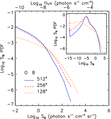
As Fig. 4, but showing the O viii flux PDF as a function of the resolution of the simulation. The particle mass (gravitational softening) increases by a factor of 8 (2) when the number of particles decreases by a factor of 23. All runs assume the same physical model, angular resolution and box size. The predictions of the N= 2563 and 5123 runs are very close for fluxes greater than 10−5 photon s−1 cm−2 sr−1.
A2 Box size
We have tested the effect of the size of the simulation box on the flux PDF of O viii emission, while keeping the resolution constant. Fig. A2 compares simulations implementing the REF model with box sizes of 100, 50 and 25 h−1 Mpc, respectively, and with constant dark matter particle mass mDM= 4.1 × 10⁸h−1 M☉. The flux PDFs converge for intermediate flux values, but diverge at the lowest fluxes. The lowest and very highest fluxes are only found in the largest box, which contains the greatest number of particles and provides the most pixels. It thus samples the tails of the distribution best.
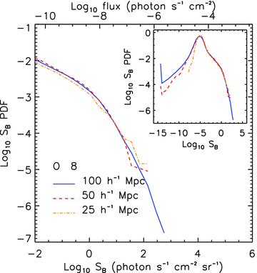
As Fig. 4, but showing the O viii flux PDF for simulations with box sizes of 100, 50 and 25 h−1 Mpc. All runs assume the same physical model, particle mass and angular resolution. Except for very low fluxes (<10−5 photon s−1 cm−2 sr−1), the results are insensitive to the size of the simulation box.
A3 Slice thickness
In this appendix, we describe how varying the thickness of the slices in which we divide the simulation box affects the flux PDF. In Fig. A3, we show this by comparing the flux PDFs, normalized by the slice thickness, for the four different, evenly spaced slice thicknesses of 40, 20, 10 and 5 h−1 Mpc.
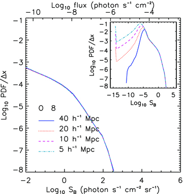
The O viii flux PDFs, normalized by the slice thickness, for maps with varying slice thickness: 40, 20, 10 and 5 h−1 Mpc. The number of slices used to calculate each PDF is 2, 5, 10 and 20, respectively. The test is for the REF model with box size 100 h−1 Mpc at z= 0.25. All maps assume the same angular resolution of 15 arcsec. In the high flux regime the PDF is proportional to the slice thickness.
In the potentially detectable regime, the results appear to be independent of the slice thickness when the flux PDF is normalized by the slice thickness. In other words, the PDF in the high flux regime is proportional to the slice thickness. This is expected if the slice is sufficiently thick to fully contain the objects giving rise to the emission, but sufficiently thin for the superposition of multiple structures to be unimportant.
The shape of the PDF at low fluxes, instead, depends on the level of the flux in low-density regions and on the number of low-density structures such as filaments that could be found in each slice, which is dependent on the slice thickness. As a consequence, the actual width of the PDF at intermediate fluxes scales with the inverse of the slice thickness and the number of pixels at the lowest fluxes increases for decreasing slice thickness.
When creating the slices, we neglect the peculiar velocities of particle, selecting them only according to their position within the simulation box. This is justified for a large slice thickness, when the peculiar velocities are small compared with the difference in the Hubble flow across the slice, because the effect of particle displacement is small. However, it may have a small effect on the predicted fluxes for the 5 h−1 Mpc slices, which corresponds to 443 km s−1 at z= 0.25.
Throughout this work, we have assumed a slice thickness of 20 h−1 Mpc, but Fig. A3 demonstrates that the results can easily be scaled to other slice thicknesses.
