


Abstract
In this paper, we revisit the issue of the propagation of warps in thin and viscous accretion discs. In this regime, warps are known to propagate diffusively, with a diffusion coefficient approximately inversely proportional to the disc viscosity. Previous numerical investigations of this problem did not find a good agreement between the numerical results and the predictions of the analytic theories of warp propagation, both in the linear and in the non-linear case. Here, we take advantage of a new, low-memory and highly efficient smoothed particle hydrodynamics (SPH) code to run a large set of very high-resolution simulations (up to 20 million SPH particles) of warp propagation, implementing an isotropic disc viscosity in different ways, to investigate the origin of the discrepancy between the theory and the numerical results. We identify the cause of the discrepancy in an incorrect calibration of disc viscosity in previous investigations. Our new and improved analysis now shows a remarkable agreement with the analytic theory both in the linear and in the non-linear regime, in terms of warp diffusion coefficient and precession rate. It is worth noting that the resulting diffusion coefficient is inversely proportional to the disc viscosity only for small amplitude warps and small values of the disc α coefficient (α≲ 0.1). For non-linear warps, the diffusion coefficient is a function of both radius and time, and is significantly smaller than the standard value. Warped accretion discs are present in many contexts, from protostellar discs to accretion discs around supermassive black holes. In all such cases, the exact value of the warp diffusion coefficient may strongly affect the evolution of the system and therefore its careful evaluation is critical in order to correctly estimate the system dynamics.
1 INTRODUCTION
Warped accretion discs may occur across a wide variety of astrophysical systems, from the large scales of accretion discs around supermassive black holes (SMBH), down to the small scales of planet forming discs.
Observationally, warps are found in galactic binary systems, such as the hyperaccreting X-ray binary SS433 (Begelman, King & Pringle 2006) and the X-ray binary Her X-1 (Wijers & Pringle 1999), and in several microquasars, including GRO J1655-40 (Martin, Tout & Pringle 2008b) and V4641 Sgr (Martin, Reis & Pringle 2008a). On the much less energetic side, a warped protostellar disc is found around the young binary system KH 15D (Chiang & Murray-Clay 2004).
Warps are also found in the thin accretion discs in active galactic nuclei (AGN), as in the case of NGC 4258 (Herrnstein, Greenhill & Moran 1996; Papaloizou, Terquem & Lin 1998). The dynamics of warped accretion can play a fundamental role in these cases, as it in turn regulates the spin history of the growing SMBH and, as a consequence, its very ability to grow rapidly (King & Pringle 2006; King, Pringle & Hofmann 2008).
The torques which produce the warp can be very different. For protostellar discs, they include tidal interactions with a companion star (Larwood et al. 1996; Martin, Pringle & Tout 2009) and dynamical effects during the formation of the disc, which might affect the relative orientation of the stellar spin and the planetary orbits (Bate, Lodato & Pringle 2010). For accretion discs around black holes there are additional torques arising from the general relativistic Lense–Thirring precession around a spinning black hole (Bardeen & Petterson 1975; Scheuer & Feiler 1996; Lodato & Pringle 2006; Martin, Pringle & Tout 2007; Perego et al. 2009; King et al. 2005) and self-induced warping caused by radiation pressure (Pringle 1996). Recently, some attention has also been given to the process of disc warping and black hole spin alignment in the case of SMBH binaries (Dotti et al. 2010). In all such cases, the evolution of the system is strongly dependent on the speed at which warping disturbances can propagate in the disc.
Analytic theories of warp propagation have been discussed extensively in the past (Papaloizou & Pringle 1983; Pringle 1992; Papaloizou & Lin 1995; Ogilvie 1999, hereafter O99; Ogilvie 2000; see Section 2). These theories predict that while for thick discs warps should propagate as dispersive waves, with a velocity of the order of half the sound speed in the disc, in the limit of thin and viscous discs the propagation is diffusive, with a diffusion coefficient inversely proportional to the disc viscosity (Papaloizou & Pringle 1983). Numerical simulations of warp propagation in the thick disc case have been performed by Nelson & Papaloizou (1999) and Nelson & Papaloizou (2000).
Numerical simulations of warp propagation for thin and viscous discs are much more challenging, because in order to properly catch the warp dynamics it is essential to accurately resolve the vertical structure of the disc, which for very thin discs can be difficult. A first attempt at testing the analytical theory with numerical simulations in the thin-disc regime has been performed by Lodato & Pringle (2007) (hereafter LP07), using smoothed particle hydrodynamics (SPH). The results of LP07 showed some unexpected results: while for large values of the disc viscosity the warp diffusion coefficient appeared to scale inversely with viscosity, as predicted analytically, such behaviour was not found at low viscosities, already for small warp amplitudes. In this case, the diffusion coefficient appeared to be much smaller than theoretically predicted, implying (as discussed extensively by LP07) some additional dissipation. Additionally, the internal precession induced by the warp and predicted analytically was found to be strongly dependent on the specific implementation of viscosity and was not found to match the theoretical expectations.
LP07 discuss different possible explanations for such disagreement. On the one hand, it is quite possible that the limited numerical resolution of their simulations might have affected their results. On the other hand, strong supersonic motions were found in the LP07 simulations, which might result into shocks in the resulting flow and thus provide the required additional dissipation.
In this paper, we want to systematically address all the issues left open by LP07, by checking both the numerical aspects of the problem and the physical effects involved.
With regard to the numerical aspects, first of all we have used a different SPH code with respect to LP07, therefore validating one code against the other. Secondly, we have checked numerical convergence by running simulations using 20 million particles, that is a factor of 10 larger than LP07 (note that such simulations are among the largest SPH simulations of accretion discs performed to date). Since some of the effects reported by LP07 appeared to depend on the viscosity formulation, we have here tested two different possible implementations of disc viscosity. Finally, we have modified our analysis procedure, so as to obtain a more quantitative evaluation of the uncertainties in the measured parameters. In order to test the physical effects which might determine the LP07 results, we have paid attention to shocks, which were argued by LP07 to be responsible for the additional dissipation. We have checked the importance of shocks by running simulations with different levels of bulk viscosity – varied independently of the shear viscosity – which is directly connected with shock dissipation.
The paper is organized as follows. In Section 2, we discuss the basic features of the analytic theory of warp propagation in both the linear and non-linear regime. In Section 3, we detail the numerical method that we have used to simulate the system, including the different implementations of disc viscosity that we use. In Section 4, we describe the procedure we have used to analyse our results and extract from the simulations the warp diffusion parameters. In Section 5, we present and discuss our main results for the warp diffusion and precession in both the linear and non-linear regime. Finally, in Section 6 we draw our conclusions.
2 ANALYTIC THEORIES OF WARP PROPAGATION
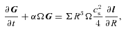
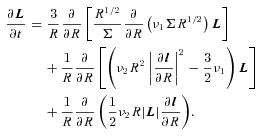
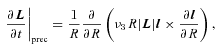
We consider here, as in LP07, the propagation of warps in thin Keplerian accretion discs, rotating with angular velocity Ω (R), with surface density Σ (R) and angular momentum per unit area L (R). Here, R should be interpreted as a ‘spherical’ coordinate. The local direction of L can be oriented arbitrarily in space and the unit vector l (R) =L (R)/L(R) defines its direction. If the disc is rotating around a central point mass M then its rotation is Keplerian, with  and
and  .
.
The disc thickness is H=cs/Ω, where cs is the sound speed, and is the scale over which density and pressure change in the local z direction. The disc aspect ratio is H/R, and we will assume that H/R≪ 1.


3 NUMERICAL METHOD
We have performed a series of three-dimensional (3D) SPH simulations of warped discs similar to, though more extensive than, those performed by LP07. SPH is a Lagrangian scheme for solving the equations of hydrodynamics in which fluid quantities and their derivatives are computed on a set of N particles that follow the fluid motion (see Price 2004; Monaghan 2005 for recent reviews).
In this paper, we have used the phantom code, developed by D. Price (see Price & Federrath 2010 for another recent application). phantom is a low-memory, highly efficient SPH code optimized for studying non-self-gravitating problems. The code is made very efficient by using a simple neighbour-finding scheme based on a fixed (in this case, cylindrical) grid and linked lists of particles. In particular, the absence of overheads associated with the tree-code for computing gravitational forces as well as other optimizations means that the code is significantly more efficient than the Benz et al. (1990)/Bate (1995)-derived code previously employed by LP07.
The initial aim of using phantom was, given the concerns in LP07, to be able to employ a much higher resolution in the calculations. Whilst in the end we found this unnecessary (see Section 5), we have instead used our increased computing ability to survey a much wider parameter space than that explored by LP07, including a wide range of viscosity parameters, two different viscosity formulations and three different warp amplitudes.
3.1 Navier–Stokes equations

 , given by
 . The corrections to Keplerian rotation due to the pressure gradient are of the order of (H/R)2, which for the thin discs considered in this paper are very small (∼ 10−4).
3.2 SPH
3.2.1 Hydrodynamics
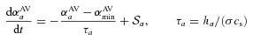
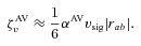
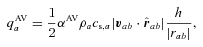
The qAV term in (23) is the AV (discussed below) which is introduced in SPH in order to capture shocks and (to a lesser extent) to prevent interpenetration of particles. However, it can be shown (see below) that the AV corresponds directly to a NS type term and can thus be used, with minor adjustment of the parameters, to directly represent physical viscous diffusion (in doing so one would obviously discard the remaining terms in equation (23), i.e. setting ζ=η= 0). The disadvantage of doing so is that the resultant viscosity coefficient consists of both shear and bulk components of viscosity, whereas for a disc the viscosity parametrization (2) should consist of shear viscosity only.
The remaining part of the SPH algorithm is the time integration algorithm, for which we use a standard leapfrog scheme equivalent to the velocity Verlet method. For efficiency, we assign individual time-steps, set in factors of 2 from a nominal maximum time-step, such that only a subset of the particles is moved on the shortest time-step. With individual time-steps many of the conservation properties of the leapfrog algorithm are only approximately satisfied; however, the scheme is significantly more efficient.
3.2.2 Artificial viscosity
 , i.e. converging flows). The signal velocity for hydrodynamics is given by
 and in general one would enforce αmax= 1.0.
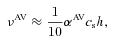
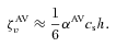
3.2.3 Disc viscosity using the AV term
 , giving
In order to use the AV to represent a Shakura & Sunyaev (1973) disc viscosity, we therefore require several minor changes from the formulation appropriate for shocks given in Section 3.2.2. These changes are as follows:
Viscosity should be applied for both approaching and receding particles;
The βAV term in the signal velocity should be dropped such that vsig=cs;
qAV should be multiplied by a factor h/| rab |, similar to the Monaghan (1992) AV scheme and
The Morris & Monaghan (1997) switch should not be used i.e. αAV should be treated as a constant.
The disadvantage of using the AV term to represent physical viscosity is that one inevitably ends up with a large and unwanted coefficient of bulk viscosity (equation 37). For a disc simulation, this is not so disadvantageous since in general ∇·v is not large, so although the coefficient is large the term to which it is applied is small. However, given that at least some of the deviations from the analytic theory found in LP07 could possibly be explained by excess dissipation, it is desirable to perform simulations that either have no explicit bulk component or where the bulk viscosity is carefully controlled as would be the case when applied to shocks in the case of the usual AV (Section 3.2.3).
3.2.4 Navier–Stokes viscosity implemented via two first derivatives
3.2.5 Navier–Stokes viscosity using direct second derivatives
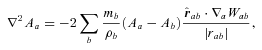
A further alternative, not considered in this paper, would be to directly evaluate the second derivative terms resulting from the gradient of the stress tensor as in equation (16), using the standard representation of second derivatives in SPH given by equations (29) and (30). Indeed this forms the basis of the ‘dissipative particle dynamics’ scheme of Español & Revenga (2003). The terms in this case are obviously similar to the formulation using AV discussed above, except that the shear and bulk components can be set separately. The disadvantage is that the total angular momentum is no longer conserved because the dissipation is not applied along the line of sight joining the particles (meaning that  ). How serious a limitation this presents in practice for disc simulations has not been clarified, though it would be worthy of further investigation.
3.2.6 Azimuthal averaging of SPH results
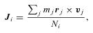

Left-hand panel: surface density profile from the SPH simulation (solid black line) and from the 1D evolution at t= 0 and 500 in code units, for the case α= 0.3, using the input value (from equation 38) (dashed green line) and the measured best-fitting value (dashed red line) of the disc viscosity for the calculation using AV to model disc viscosity at an SPH resolution of 2 million particles. We find very close agreement between the input and fitted values. Right-hand panel: same, but using NS viscosity. In this case, the fit with the Σ profile is slightly better, giving smaller error bars in the fitted value of α.
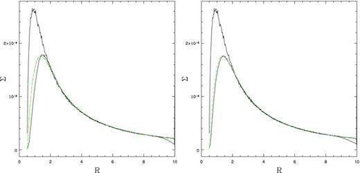
Evolution of the shell averaged profiles of lx from the SPH simulations at t= 0 and t= 500 in code units (solid black lines), for the low-viscosity case α= 0.065 and A= 0.01, compared to the results of a 1D evolution assuming wave-like propagation with dissipation at the appropriate value of α, from equations (3) and (4) (dashed red lines). The excellent agreement explains the deviations at low α seen in Fig. 5, as been due to the transition to the wave-like propagation regime at low viscosity.
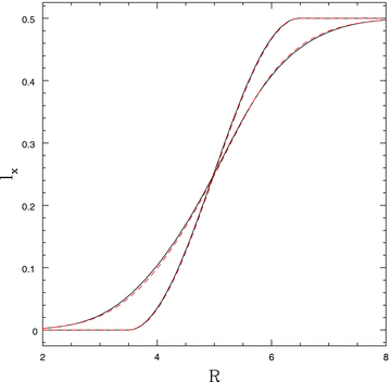
Shell averaged profiles of lx from the SPH simulation (solid black lines) at t= 0 and 1000 (in code units), compared to the corresponding profiles from the diffusive evolution, for the high-viscosity case α= 0.43 and a strongly non-linear warp amplitude (A= 0.5), assuming the warp diffusion coefficient to be a function of α and ψ, as predicted by O99 (dashed red lines).
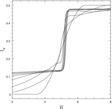
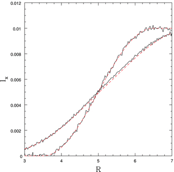
Shell averaged profiles of lx from the SPH simulation (black lines) at intervals of Δt= 500 up to t= 3500 (in code units), for the low-viscosity case α= 0.03, using 20 million particles and a strongly non-linear warp amplitude (A= 0.5). The large warp amplitude simulations at low α show a strong steepening effect in the warp profile because different parts of the warp propagate at different speeds. A comparison with the non-linear theory is more difficult in this case because the predicted diffusion parameter for the disc can become negative, causing unphysical oscillations in the 1D code.
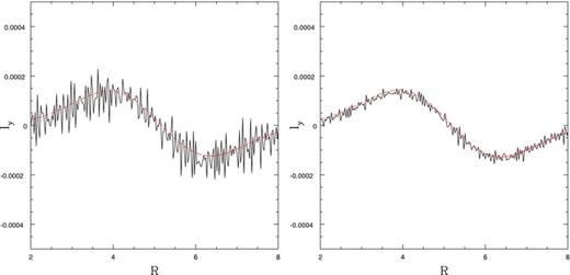
Left-hand panel: profile of ly at t= 1000 (in code units) for the α= 0.43 case. The solid black line shows the SPH results at a resolution of 2 million particles. The dashed red line shows the expected profile from the diffusion plus precession equation with the fitted value of α3. Right-hand panel: profile of ly at t= 1000 code units for the α= 0.46 case, at an SPH resolution of 20 million particles (lines are the same as for the left-hand panel).
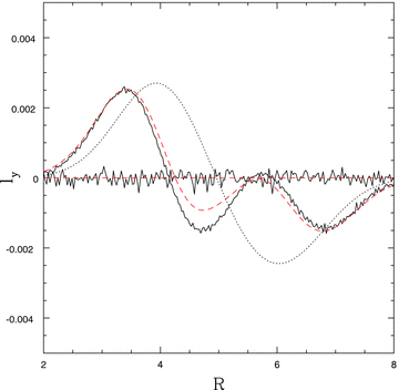
Profile of ly at t= 500 time units for the case A= 0.5 and α= 0.43. The solid black lines refer to the SPH simulations, while the dashed red line shows the result of the evolution of the diffusion plus precession code, with non-linear warp parameter α2 and α3 computed based on the O99 theory of warp propagation. For comparison, we also show with the dotted black line the profile at t= 500 obtained from the simple 1D evolution model assuming a constant α3= 0.22, appropriate for this value of α in the linear regime (ψ≪ 1).
3.3 Initial conditions
Initial conditions are identical to those in LP07. We use code units in which the gravitational constant G= 1, the central point mass M= 1 and the time unit is such that at a radius R= 1 (in code units) the dynamical time is Ω−1= 1. We place the gas particles in Keplerian orbits in the gravitational potential of a point mass with M= 1 (in code units). The gas particles are removed from the calculation inside a radius R= 0.5 (in code units). We distribute the particles using a Monte Carlo placement method such that the disc has a prescribed initial surface density profile, as described below. The particles are distributed in z so as to attain a Gaussian density profile in the vertical direction, with thickness H=cs/Ω. The random particle placement, whilst simple, means that some settling of the disc occurs during the first few dynamical times of the simulation.


A 3D rendering of the resulting warped disc from one of our high-resolution (20 million particle) calculations is shown in Fig. 1, for the case of a high amplitude warp (A= 0.5). A cross-section of the disc in a 2 million particle simulation with a low amplitude warp (A= 0.01) is shown in Fig. 2, showing the slight bend induced in the disc profile. The initial shape of the warp is also plotted in fig. 1 of LP07 and is shown by the lines corresponding to t= 0 in Figs 7 and 9 of this paper.
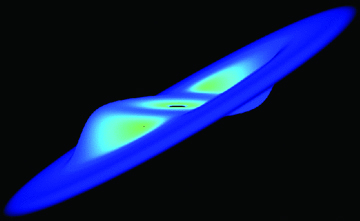
3D structure of the warped accretion disc from a representative 20 million particle calculation in the large warp amplitude case (A= 0.5).

Cross-section of the disc in the SPH calculations for a low amplitude warp (A= 0.01) at a resolution of 2 million particles.
We choose the normalization of the sound speed such that the aspect ratio of the disc at R0= 5 is H/R= 0.0133, corresponding to an aspect ratio at R= 1 (in code units) of H/R= 0.02, in order to model a thin disc, where warps propagate primarily in the diffusive regime (see Section 2).
4 ANALYSIS
4.1 1D Disc evolution
We compare the time evolution of Σ and l from the SPH simulation with the one resulting from equation (5). This is solved using standard finite difference methods, which are detailed in Pringle (1992) and LP07, but with a different implementation of the zero-torque boundary condition at the inner edge. While in Pringle (1992) and LP07 the zero-torque condition is implemented in an approximate way, by artificially removing mass from the innermost cells in order to keep Σ close to zero, in this paper we directly enforce Σ= 0 at the innermost cell. The two conditions are largely equivalent, but the shape of the surface density profile in the inner disc can be slightly modified. This is important because in turn it significantly affects the evaluation of α, as described in Section 5.1.
4.2 Fitting procedure
The main aim of this paper is to determine the relation between the two parameters α and α2, which describe the disc viscosity and the warp diffusion coefficient, respectively. In principle, the parameter α should be simply determined by the input viscosity coefficient in the SPH code as per Section 3.2. However, LP07 did not find a perfect match between the nominal value of α as expected from the continuum limit of SPH and the α measured from the 1D surface density evolution using equation (5), and therefore preferred to fit both parameters independently, to get the desired relation. In particular, LP07 ‘stress that [they] do not perform an actual statistical fit of the viscosity coefficients, but simply choose them so as to match the evolution of the numerical simulation’. This point is discussed further in Section 5.1.
In this paper, we have implemented a statistical fitting procedure to check the calibration between the input α parameter and the value measured from comparing the SPH and the 1D evolution of the disc using (5). The same procedure is further used to measure the warp diffusion coefficient α2 and the precession coefficient α3. This procedure is described below. Specific results for the calibration of α and the estimate of α2 and α3 are reported in Section 5.
4.2.1 Fittting for α
An example of the best-fitting Σ profile compared to the averaged SPH profile is shown in Fig. 3. As it turns out, the best-fitting profile is in fact very close to the one computed using the input value for α, so this fitting procedure for α itself becomes unnecessary (see Section 5.1, below).
4.2.2 Fittting forα2andα3
The values of α2 and α3 are obtained using a similar procedure, though the computation of either requires, and is dependent on, an input value for the disc viscosity α– i.e. using either the nominal or fitted α value.
 using a scheme analogous to the one used for α.
5 RESULTS
The initial aim of this paper was to perform simulations at a resolution significantly higher than that employed by LP07, in order to assess the effect of limited resolution. Having performed several calculations with 20 million SPH particles and finding results indistinguishable from the lower resolution of 2 million particles, we have instead surveyed a wide range in parameter space, performing a total of 78 simulations using 2 million particles together with the original eight at 20 million particles. These consist of eight series of simulations, each for a range of viscosity values. The parameters for each series are given in Table 1, where we have considered the effect of resolution (2 versus. 20 million particles), three different warp amplitudes (A= 0.01, 0.05 and 0.5), disc viscosity formulated either using the modified AV or by a direct implementation of NS terms, considering the latter with zero bulk viscosity and subsequently with a small amount applied using a switch.
Parameter settings for each of the eight series of calculations performed in this paper, where each series consists of a set of simulations covering a range of disc viscosities α. The second column gives the initial warp amplitude A used in equation (43), the third column shows whether the disc viscosity was represented using the modified AV term or via a direct implementation of NS viscosity. The fourth column shows whether or not bulk viscosity was applied (always true for the AV calculations). The resolution of the calculations is given in the fifth column and the symbols used to represent each series in Figs 4, 5, 6, 8 and 13 are given in the last column.
| Series | A | Visc. type | Bulk visc.? | Npart | Symbols |
| 1 | 0.01 | AV | Yes | 2 × 10⁶ | Red triangles |
| 2 | 0.05 | AV | Yes | 2 × 10⁶ | Orange triangles |
| 3 | 0.01 | AV | Yes | 2 × 10⁷ | Green triangles |
| 4 | 0.05 | AV | Yes | 2 × 10⁷ | Cyan triangles |
| 5 | 0.01 | NS | No | 2 × 10⁶ | Black squares |
| 6 | 0.01 | NS | Switch | 2 × 10⁶ | Blue squares |
| 7 | 0.5 | AV | Yes | 2 × 10⁶ | Magenta triangles |
| 8 | 0.5 | AV | Yes | 2 × 10⁷ | Yellow triangles |
5.1 Calibration of the disc viscosity coefficient
The best matching values of α (here referred to as αfit) reported in Table 1 of LP07 do not follow the expected relation given by equation (38). Although, for a given 〈h〉/H, the relation between αfit and αAV is approximately linear, the slope is shallower than expected. An accurate calibration of α is important, because in turn it is used as an input for the evaluation and fitting of the warp diffusion coefficient α2. The disagreement found in LP07 prompted us to examine the method used to calibrate α in greater detail, resulting in our implementation of the fitting procedure described in Section 4.2– essentially a quantitative version of the procedure performed in LP07.
In considering this issue, we have also explored the effect of the inner boundary condition of the 1D disc evolution on the measurement of α. Indeed, the main feature which is used for the evaluation of α is the turnover of the surface density at small radii, which might well be affected by the specific boundary condition used. Using the same condition employed by LP07 (described in Section 4.1), we found a similar relationship between αfit and αAV– i.e. not matching the expectations from equation (38). Furthermore, we found that the calculations using a NS viscosity also did not agree with the measured values. However, when the zero-torque boundary condition was enforced exactly (see Section 4.1), the disagreement was removed. This is demonstrated in Fig. 4, which shows the best-fitting value αfit versus the input value of α calculated using equation (38). Results are shown with triangles for the calculations where the disc viscosity has been simulated using the SPH AV, whilst squares correspond to calculations where NS viscosity terms have been implemented directly. All calculations are performed at a resolution of 2 million SPH particles, except for the green and cyan triangles that use 20 million particles. The error bars show the 1σ errors from the fitting procedure.
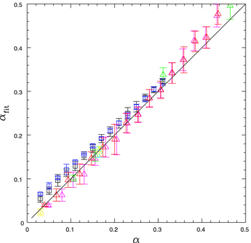
Comparison between the input value of α and the measured value obtained fitting the SPH data to the 1D evolution of Σ, with the zero-torque boundary condition enforced exactly. Results are shown with triangles for the calculations where the disc viscosity has been simulated using the SPH AV, whilst squares correspond to calculations where physical viscosity terms have been implemented directly. All calculations are performed at a resolution of 2 million SPH particles, except for the green, cyan and yellow triangles that use 20 million particles. Error bars refer to the 1σ errors from the fitting procedure used to obtain αfit.
As one can see from Fig. 4, the general agreement is very good. In other words, the procedure used by LP07 to simultaneously fit α and α2 is no longer necessary and henceforth we simply fit the single parameter α2 using the input value for α.
Also worth noting from Fig. 4 is that whilst the error bars are smaller using the NS viscosity (squares) – due to an improved agreement of the profile of Σ near the inner boundary (see the right-hand panel of Fig. 3) – there appears to be a small excess dissipation that occurs for low input α. In the case of Series 5 (black squares), this may be naturally attributed to the small amount of AV we have applied. However, for Series 6 (blue squares), using zero AV paradoxically results in an even greater dissipation. We attribute this to the increased randomness of the particle distribution arising when no bulk viscosity is present. A similar effect is seen in several other SPH simulations, e.g. in Price & Federrath (2010) when βAV is too low.
5.2 Results for the warp diffusion coefficient
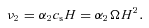
The results of the fitting procedure for the warp diffusion coefficient α2 are shown in Fig. 5, for Series 1–5 discussed above. The solid line in the figure shows the simple relation α2= 1/(2α) expected in the linear regime of warp propagation discussed in Section 2 (Papaloizou & Pringle 1983). What is most striking is that the numerical results do not appear to match the 1/(2α) relation in almost any regime. In particular, at high α, the measured values of α2 lie much above the simple 1/(2α) relation, while at low α they lie slightly below it. This is contrary to the result shown in LP07, where agreement was found at high α, and a much larger disagreement was found at low α. The origin of the discrepancy between our results and those of LP07 lies in the more accurate evaluation of the disc viscosity α discussed above and the resultant effect on the fit for α2.
Relation between the warp diffusion coefficient α2 and the disc viscosity α, for warp amplitudes A= 0.01 (black squares, red and green triangles) and A= 0.05 (orange and cyan triangles). Squares use a direct implementation of the NS terms, whilst triangles use the SPH AV to represent the disc viscosity. All calculations employ 2 million SPH particles, except the cyan and green triangles, which use 20 million. The solid line shows the simple α2= 1/(2α) relation from Papaloizou & Pringle (1983). The long-dashed line includes the non-linear corrections due to finite values of α for small amplitude warps (equation 8).
The natural question is therefore why do the new, more accurate results not agree with the standard theory?
Initially, we will discuss only the simulations with a small warp amplitude A= 0.01. The effect of finite warp amplitude is discussed later in Section 5.2.5
5.2.1 Effect of resolution
Our first attempt to reconcile the simulation with the theory was to check for resolution effects. In particular, these are thin discs, and the vertical scaleheight is only moderately resolved (by only 1.6 smoothing lengths) at a resolution of 2 million particles (see Fig. 2). LP07 also mention the possibility of resolution effects in their simulations (which have the same resolution of 2 million particles) but nevertheless demonstrate that the vertical density profile is very well reproduced (see fig. 2 of LP07), and hence argue that such effects should be negligible. We have therefore performed six calculations at the higher resolution of 20 million particles (four with A= 0.01 and two with A= 0.05), for which the vertical scaleheight is resolved with ∼3.5 smoothing lengths. The results of these higher resolution simulations are shown with green and cyan triangles in Fig. 5 and show no significant difference with respect to the lower resolution case. Note that the calibration of α for these calculations, shown in Fig. 4, is very similar to the 2 million particle case, despite the very different smoothing lengths. We therefore conclude that resolution effects are not to blame for the discrepancy.
5.2.2 Effect of viscosity formulation
The results of LP07 showed strong disagreement with the standard theory at low α. LP07 argue that a discrepancy between their results and the standard theory at low α might arise because of enhanced dissipation due to the presence of supersonic motions and hence shocks. With the recalibration of α discussed above, the disagreement at low α is significantly reduced and, as we show later, can now be explained by the transition to the wave-like propagation regime.
Nevertheless, when using the SPH AV to represent disc viscosity, one inevitably ends up with a large bulk viscosity coefficient (see Section 3.2.3, equation 37), which could perhaps explain the excess dissipation invoked by LP07. In order to check whether bulk viscosity affects the magnitude of the warp diffusion coefficient, we have implemented a full NS viscosity, as described in Section 3.
The results of the calculations using the NS viscosity and zero bulk viscosity and the AV set to zero are shown in Fig. 6 (blue squares), and indeed appear to show a significant effect, lowering the measured values of α2 at low α. But, as discussed in great detail in LP07, this implies an even greater excess dissipation. Thus, paradoxically, by removing bulk viscosity we have apparently increased the amount of dissipation present in the simulation. However, some caution is required here, since – as discussed in section 3.2.4– one should be very careful about completely removing all bulk viscosity from SPH simulations, since it plays a necessary role in preventing particle interpenetration, as well as providing physical dissipation in shocks, if shocks are present.
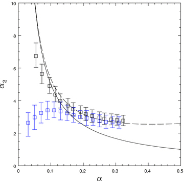
As in Fig. 5, but comparing only the two series using NS viscosity, with (black suqares) and without (blue squares) a small amount of artificial bulk viscosity. Despite the nominally lower input viscosity, the calculations with zero bulk viscosity paradoxically show a larger dissipation, as evidenced by the lower magnitude of the warp diffusion coefficient α2. We attribute this to the danger of using zero bulk viscosity in SPH.
We have therefore also computed a series of simulations with NS shear viscosity, but with a small amount of AV, applied only for approaching particles and using a switch to reduce its amplitude away from shocks (black squares in Figs 5 and 6). Note that the effective bulk viscosity coefficient in this case is much smaller (at least a factor of 5) than that present in the simulations that use AV to represent disc viscosity (i.e. the red triangles in Fig. 5). Despite the very small change in the viscosity formulation, the results of this series of simulations (series 5, black squares in Fig. 5) are in very good agreement with those presented previously (Series 1, red triangles). This leads us to conclude that the dramatic effect produced in Fig. 6 by removing all of the bulk viscosity is most likely a numerical artefact. This is strengthened by the results already discussed in Fig. 4, also showing that the simulations with zero bulk viscosity show a higher dissipation, that can be attributed to the increased randomness of the particle distribution when no bulk viscosity is present.
5.2.3 Are we looking at the right theory?
Having investigated the effect of both resolution and viscosity formulation, we may dispense with the possibility that the disagreement between the SPH simulations and the simple linear theory is simply a numerical artefact. What is worse, the recalibration of α discussed in Section 5.1 puts us in a worse position than LP07, as we now disagree with the linear theory at both low and high values of α, contrary to the results of LP07, where the results appeared to agree at high α. In our case, the results are also more significant, because we have much better statistics (86 simulations compared to the 10 shown in fig. 8 of LP07), spanning a wider range in all of the parameters α, α2 and the warp amplitude.
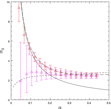
Relation between the warp diffusion coefficient α2 and α for large amplitude warps. The magenta triangles show the results for A= 0.5, while the red triangles, for comparison, indicate the small amplitude (A= 0.01) case. The solid and long-dashed lines show the 1/(2α) relation and the corrections expected for finite α, respectively. The short-dashed line shows the expected relation based on the non-linear theory of O99, assuming a fixed ψ= 0.55 (roughly comparable to the average ψ value using A= 0.5). The large error bars in the high-amplitude case at low α are because the non-linear warp evolution is not well fitted by a single value for α2– physically manifested as a steepening of the warp profile observed in the simulations (see Fig. 10) that is not captured by the fitted linear profiles.
Clearly, though, the α values we are using here at not small, and therefore it may well be expected that the nominal 1/(2α) relation is not appropriate, particularly at the high-α end of our parameter range. Indeed, when we plot the relation between α2 and α predicted for finite values of α by equation (8) (long-dashed line in Figs 5 and 6), we recover an excellent agreement with the SPH results for α≳ 0.15 for low-amplitude warps.
We thus conclude that there is no disagreement between our numerical results at high α and the linear theory of warp propagation, once the effects of finite α are appropriately accounted for in the theory. The only remaining issue is a small disagreement at low α for small amplitude warps – though much smaller than the one found in LP07, which we discuss in the next section.
5.2.4 Low-viscosity behaviour and transition to the wave-like propagation regime
In principle, there could be two explanations for the remaining small disagreement that we find for low viscosity: a numerical one, related to our procedure to fit the value of the diffusion coefficient α2, and a physical one, related to an actual transition to a different propagation regime, such as the wave-like propagation regime (Section 2).
There are good reasons to believe that both effects might play a role for small values of the viscosity coefficient. From the numerical point of view, we note that our fitting procedure is based on matching the solution of the simple diffusion equation to the SPH results at a given time, t= 1000 in code units, which corresponds to 0.4α in units of the viscous time at R= 1. The viscous time is not only a measurement of the time needed for the overall viscous evolution of the disc to take place but also of the time needed to smooth out the discreteness of the particle distribution in the initial condition. We therefore might expect that, for small α, the SPH simulation at t= 1000 code units is still somewhat noisy, and that it might affect the evaluation of α2. That this is the case can already be seen from the fact that the error bars on α2 get larger at small α. Additionally, we have also found that for small α the results are somewhat sensitive to the time at which the fit is performed. If the fit is performed at earlier times, the resulting value of α2 tends to be systematically shifted down by a small amount.
The results of the calculation for low α might also be affected by the fact that warp propagation undergoes a transition to the wave-like regime (Section 2), which, for small warp amplitudes, is expected to occur at around α≲ 2πH/λ≈ 0.07, where λ is the wavelength of the perturbation (which in our case is λ∼ 6 in code units). In order to test this hypothesis, we compare the evolution of the SPH simulation to the 1D evolution appropriate to the wave-like regime (equations 3 and 4), including dissipation corresponding to the input value of α from the simulation. The results of this test are shown in Fig. 7 for a low amplitude warp with α= 0.065, from Series 1. The plot shows the profile of the x-component of the unit vector l from the SPH simulation at t= 0 and 500 in code units (solid black lines) compared to the 1D evolution from equations (3) and (4) (dashed red lines). The fact that the profiles agree well indicates that wave-like propagation, albeit with diffusion, can explain the deviation from the purely diffusive propagation we have assumed when comparing with equation (7) or (8).
Given that there is no longer any disagreement between theory and the results of the SPH simulations, contrary to LP07, it is no longer necessary to invoke any additional dissipation involved in warp propagation.
5.2.5 Large amplitude warps
Having gained some confidence that the linear theory of warp propagation explains satisfactorily the evolution of the SPH simulations at low warp amplitudes, we may turn our attention to non-linear effects.
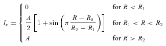
Initially, we have considered a small increase in the initial warp amplitude to A= 0.05 in equation (43). The results of these calculations (Series 2) are shown with orange triangles in Fig. 5 and are essentially indistinguishable from the A= 0.01 case (Series 1 and 5), demonstrating that the linear theory is applicable also in this case.
The resulting values of α2 from our fitting procedure for the A= 0.5 case (Series 7) are shown in Fig. 8 with magenta triangles, compared to the corresponding Series 1 for A= 0.01 (red triangles). One can immediately see that the fitted values of α2, for small α, are much smaller than the low amplitude case, and are characterized by a much larger uncertainty.
At very large warp amplitudes, the linear theory of warp propagation in the diffusive regime is not applicable, and it is therefore not surprising that, indeed, the SPH simulations in this regime (A= 0.5) do not match either the 1/(2α) relation or the more complete relation of equation (8) which is non-linear in α but assumes linearity in the warp amplitude. O99 presents a non-linear theory of warp propagation for warps of any amplitude. We are now in a position to test this theory numerically.
The complicating factor is that, in the O99 theory, α2 is a function of the warp amplitude ψ (related to A by equation 46, with the maximum value given by equation 47). We thus cannot associate a single value of α2 to each large amplitude simulation, as ψ is a function of radius (equation 46) and furthermore decreases as a function of time as the warp diffuses. Indeed, this is the reason for the large error bars in Fig. 8 when attempting to fit a single α2 value to the lx profile, particularly at low α where in the O99 theory the dependency of α2 on ψ is much stronger. What is possible is to check whether the deviations expected from such non-linear theory follow the observed trend, i.e. a general decrease of the diffusion coefficient. The short-dashed line in Fig. 8 shows the relation between α2 and α based on the theory of O99 for a fixed value of ψ= 0.55, computed numerically based on a routine kindly provided to us by Gordon Ogilvie. We can indeed see that the non-linear theory does reproduce qualitatively the observed trend.
As an additional test of the theory, we have also evolved the standard equation for diffusive evolution (equation 5), where the diffusion coefficients α1 (now different from α) and α2 are computed at each radius and at each time-step, based on Ogilvie’s non-linear theory. In this case, we do not have any free parameter to fit: α is the nominal value of the viscosity coefficient, and α1 and α2 are prescribed functions of α and ψ which we compute at each radius and time by evaluation of the relevant integrals in O99 using the routine provided. The resulting profiles of lx are shown in Fig. 9 for the case where α= 0.43. The black solid lines show the results of the SPH simulations at t= 0 and 1000 (in code units), while the red dashed line show the corresponding profiles computed from equation (5). The agreement of the non-linear theory with the SPH results is excellent. Note that the warp diffusion coefficient in the theory of O99 depends also on the amount of bulk viscosity present in the disc. Indeed, in order to get the good match shown in Fig. 9 we have computed the warp diffusion coefficient assuming a bulk viscosity with magnitude αb= 5α/3, as expected from the SPH formalism (see Section 3.2.2).
At low disc viscosities (small α), the simulations show a steepening effect in the warp profile – the physical result of different parts of the warp propagating at different speeds. We find that the steepening becomes stronger as the disc viscosity is reduced (evident from the increase in the error bars seen in Fig. 8 as α→ 0) and in the limit of extremely small viscosity can result in a near-complete break in the disc. This is demonstrated in Fig. 10 which shows the equivalent of Fig. 9 for a low-viscosity calculation (α= 0.03) shown at intervals of t= 500 in code units and evolved as far as t= 3500. A 3D rendering of the disc structure is shown in Fig. 11 at t= 1500 in code units. Despite the apparent break, the calculations are able to resolve a thin but steady stream of material continuing to accrete across the discontinuity, indicating that the disc regions remain connected even in this extreme case.
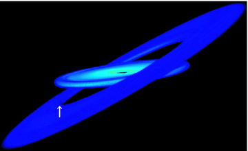
Resulting 3D disc structure from the simulation shown in Fig. 10 with a large amplitude warp in a low-viscosity disc (α= 0.03), shown at t= 1500 (in code units). The steepening of the warp profile in this case results in a nearly complete break in the disc. At the employed resolution of 20 million particles, we are able to resolve the thin but steady stream of material that is nevertheless still being transported inwards across the discontinuity (just visible in the figure, as indicated by the arrow).
 , which is the case here) the effective viscosity becomes negative, suggesting that diffusion is no longer an appropriate description. Whilst for small amplitude warps one expects a transition to the wave-like regime at low α (based on the dispersion relation derived from the linear wave equations, equations 3 and 4), it is not clear from theory at which value of α the transition occurs for large amplitude warps, and indeed whether such a transition occurs at all if ψ is sufficiently large (Ogilvie, private communication). Furthermore, calculations by Ogilvie (2006) based on the evolution of a 1D non-linear Schrödinger equation for inviscid, Keplerian discs suggest that wave-like propagation should not have a steepening effect for an isothermal equation of state (more specifically, if the adiabatic index γ < 3), suggesting that the steepening we observe is indeed a diffusive rather than wave-like effect, though it is hard to be certain in the absence of a full non-linear theory for wave-like propagation.
5.3 Precession
The last remaining piece of the theory which needs to be tested is the one related to precession. As mentioned in Section 2, the full theory of warp propagation presented in O99 predicts also the presence of internal precessional torques. These can be accounted for within the simple diffusion model of Pringle (1992) (equation 5) by adding an appropriate additional term (equation 9). We have included such terms and fitted the value of the corresponding new parameter α3 to the SPH data. In this case, the disc property which relates to precession and that we use to perform the fit is the profile of the y-component of the angular momentum in the disc ly.
Fig. 12 shows the profiles of ly at t= 1000 code units (solid black lines) and the corresponding solution of the diffusion equation with added precessional term, using the fitted value of α3 (dashed red lines). The left-hand panel refers to α= 0.43 and an SPH resolution of 2 million particles, while the right panel refers to α= 0.46 and an SPH resolution of 20 million particles. Note that the amplitude of the induced precession – and therefore of the value of ly– is small, and therefore the SPH data are quite noisy for ly, especially at low SPH resolution. This implies a rather large uncertainty in the fitted value of α3.
The resulting values of α3 as a function of α are plotted in Fig. 13 for Series 1–4 (i.e. for the small amplitude cases with disc viscosity modelled through the AV term). Given the large uncertainty at the lower resolution and lowest warp amplitude (A= 0.01), error bars are shown only for the A= 0.05 and higher resolution calculations for clarity (by way of comparison the error bars for the low-resolution A= 0.01 calculations are roughly a factor of 2 larger than for the corresponding low-resolution A= 0.05 results). The solid line shows the small amplitude and α≪ 1 approximation α3= 3/8 (equation 10), whilst the long-dashed line gives the expected relation for small warp amplitudes but to higher order in α (equation 11). Once again, provided the corrections for finite α are accounted for, we obtain a very good agreement between our numerical results and the theory, except for the lowest values of α. The deviations seen at low α are most likely due to the effect of bulk viscosity in the code which affects the ly profile more strongly than either lx or lz (simply due to the low amplitude of ly) and is more significant when the disc viscosity is low.
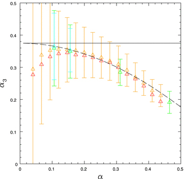
Relation between the precession coefficient α3 and the disc viscosity α, for warp amplitudes A= 0.01 (red and green triangles) and A= 0.05 (orange and cyan triangles). All calculations employ 2 million SPH particles, except the cyan and green triangles, which use 20 million. The solid line shows the expected precession rate in the limit of small α, while the dashed line shows the relation between α3 and α expected for small amplitude warps from the theory of O99 (equation 11).
We note briefly that – by contrast with our earlier results for both α and α2– the calculations utilizing the NS implementation of viscosity (Series 5 and 6) show a strong disagreement with both the modified AV calculations and the theoretical curves – the precession even reversing direction for α≲ 0.07. The fits for series 6 – i.e. the calculations that show good agreement in the α2 fits – show the fit to α3 rise with α (from negative values) and then flatten to around α3≈ 0.23 at α≳ 0.2, in contrast to the results shown in Fig. 13. The results for Series 5 show a similar trend but with much lower fitted values. The errors to the fits are also significantly larger than for the AV calculations. Whilst we can only speculate as to the reason for this disagreement, most likely it is an indication that higher resolution is needed (compared to using the modified AV) to evaluate the nested first derivatives (equations 39 and 13) to the accuracy required in order to measure the precessional contribution. LP07 also found the precession in their simulations to depend strongly on details of the viscosity formulation.
Finally, let us consider the internal precession for large amplitude warps (A= 0.5, Series 7). In this case, as for the evaluation of the warp diffusion coefficient, we cannot simply associate a single value of α3 to our simulation, as it depends on the instantaneous value of ψ, which is a function of R and t. However, we can still compare the profile of ly at a given time to the one expected from the non-linear theory of O99. Once again, we stress that in this comparison we have not fitted any parameters, as the value of α is simply the input value in the simulation, while both α2 and α3 are a prescribed function (obtained from O99) of α, αb= 5α/3 and ψ. The profile of ly for α= 0.43 and A= 0.5 is shown in Fig. 14 at t= 0 and 500 (in code units). The solid black lines show the results of the SPH simulations while the dashed red lines refer to the solution of the diffusion equation with added precession, where the coefficients are computed directly from the non-linear theory of O99. Note that, while in this large amplitude case the resulting shape of ly is a more complicated function than a simple oscillating function (as in the small amplitude case), the profile is reproduced surprisingly well by the O99 theory. To emphasize the importance of non-linear effects in this case, we also show with the dotted black line in Fig. 14 the profile of ly at t= 500 obtained from the 1D evolution code neglecting the effects of non-linearity and simply adopting a constant α3= 0.22 that is the value of the precession coefficient for α= 0.43 in the small amplitude limit. One can thus clearly see that the non-linearity in the determination of α3 is essential in order to reproduce the correct precession of the disc.
6 CONCLUSIONS
In this paper, we have numerically tested the non-linear propagation of warps in thin and viscous accretion discs. To this end, we have run very high resolution SPH simulations of warped accretion discs, extending the previous work of LP07 to cover a much wider region of the parameter space. In some simulations, we have increased the numerical resolution with respect to LP07 by using 10 times as many particles. We have also checked the effect of two different implementation of the disc viscosity.
Our new and improved results correct upon the previous results of LP07, who had found a disagreement between their simulations and the analytical theories of warp propagation. On the contrary, our results are in spectacular agreement with the non-linear theory of warp propagation of O99. Some specific features of this theory, confirmed by our simulations, are worth recalling as follows.
For moderate values of α≳ 0.1, the warp diffusion coefficient ν2 is not proportional to 1/α, where α is the disc viscosity coefficient, but follows the slightly more complex relation (equation 8). The ‘standard’1/α behaviour is only recovered for smaller values of αand for small amplitude warps. Note that a value of α≈ 0.1 is expected based on observations of accreting binary systems (King, Pringle & Livio 2007).
For large amplitude warps, the relation between ν2 and ν is much flatter than the 1/α relation, corresponding to a more uniform (with respect to the disc viscosity) but also much less efficient diffusion of the warp at low α compared to the linear case. Our simulations, which are characterized by a warp amplitude ψ≈ 1 are reasonably well described by an almost constant α2≈ 2.5.
In general, for non-linear warps, the warp diffusion coefficient is a function of the warp amplitude, which is itself a function of position and time. For a proper calculation of the warp evolution in a simple 1D diffusion code, it is essential to include such dependence. We stress that this can and should be done in any warp diffusion code.
The non-linear theory also predicts the appearance of internal precessional torques. Also, such torques are well described by the non-linear theory of O99 and can be easily included in 1D models by the simple addition of an extra term in the evolution equation, as discussed in the text.
For large warp amplitudes and small viscosity (
 ), the evolution of the system is not well described by a simple diffusion equation and a full numerical approach is thus needed in such cases.
All of the above aspects of warp propagation are reproduced faithfully in our simulations and can deeply affect the structure and evolution of the disc. We stress that their implementation (except for the last point) is relatively easy and recommended in simple 1D models of warped accretion disc evolution.
Before concluding, we should add a word of caution. All of the above results refer to warp propagation in a disc where viscosity is a standard NS viscosity, and in particular to the case where it is isotropic. Accretion disc viscosity is generally thought to be due to turbulence driven by some disc instability, such as the magnetorotational instability (Balbus & Hawley 1991) or gravitational instabilities (Lodato & Rice 2004; Lodato 2007). In such cases, it is not obvious that the induced transport can be described in terms of an isotropic viscosity coefficient, and some of the above results, in particular concerning the precessional terms (LP07), might be affected.
Note that this is given incorrectly as 3/4 in Papaloizou & Pringle (1983) and correspondingly in LP07.
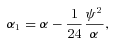
The reader should note that O99 uses a slightly different notation, defining the coefficients using Q1≡− 3α1/2, Q2≡α2/2 and Q3≡α3.
We thank Jim Pringle for several stimulating discussions and Gordon Ogilvie for providing us with the routine to compute the non-linear warp coefficients and for helpful comments on the paper. GL acknowledges the support of the Isaac Newton Institute for Mathematical Studies, where some of this work has been carried out. DJP acknowledges the support of a Monash fellowship. A substantial part of this work was also completed whilst DJP was funded by a UK Royal Society University Research Fellowship. Calculations were performed on zen, the SGI Altix ICE supercomputer at the University of Exeter and the Monash Sun Grid. DJP thanks Dave Acreman at Exeter and Philip Chan and the e-Research Centre at Monash for ably managing the respective facilities. Figs 1, 2 and 11 were produced using splash (Price 2007), a visualisation tool for SPH data.
REFERENCES
