


Abstract
We present data products from the Canada–France–Hawaii Telescope Lensing Survey (CFHTLenS). CFHTLenS is based on the Wide component of the Canada–France–Hawaii Telescope Legacy Survey (CFHTLS). It encompasses 154 deg2 of deep, optical, high-quality, sub-arcsecond imaging data in the five optical filters u*g′r′i′z′. The scientific aims of the CFHTLenS team are weak gravitational lensing studies supported by photometric redshift estimates for the galaxies. This paper presents our data processing of the complete CFHTLenS data set. We were able to obtain a data set with very good image quality and high-quality astrometric and photometric calibration. Our external astrometric accuracy is between 60 and 70 mas with respect to Sloan Digital Sky Survey (SDSS) data, and the internal alignment in all filters is around 30 mas. Our average photometric calibration shows a dispersion of the order of 0.01–0.03 mag for g′r′i′z′ and about 0.04 mag for u* with respect to SDSS sources down to iSDSS ≤ 21. We demonstrate in accompanying papers that our data meet necessary requirements to fully exploit the survey for weak gravitational lensing analyses in connection with photometric redshift studies. In the spirit of the CFHTLS, all our data products are released to the astronomical community via the Canadian Astronomy Data Centre at http://www.cadc-ccda.hia-iha.nrc-cnrc.gc.ca/community/CFHTLens/query.html. We give a description and how-to manuals of the public products which include image pixel data, source catalogues with photometric redshift estimates and all relevant quantities to perform weak lensing studies.
1 INTRODUCTION
Our knowledge of the nature and the composition of the Universe has evolved tremendously during the past decade. A combination of observations has led to the conclusion that the Universe is dominated by a uniformly distributed form of dark energy. Chief pieces of evidence for this conclusion are that the expansion rate is accelerating (from the distances to supernovae; see e.g. Riess et al. 1998, 2007; Perlmutter et al. 1999), that the Universe is flat (from the cosmic microwave background; see e.g. Komatsu et al. 2011) and that dark matter cannot provide the critical density (for instance through galaxy cluster studies; see e.g. Allen, Evrard & Mantz 2011). As the standard accelerating Universe is set on such solid grounds, one of the main goals of cosmology is now to get a precise understanding on the nature of dark matter and dark energy.
Complementary to the observations mentioned above, weak gravitational lensing has been recognized as one of the most important tools to study the invisible Universe. Inhomogeneities in the mass distribution cause the light coming from distant galaxies to be deflected which leads to a direct observable distortion of galaxy images. Because the lensing effect is insensitive to the dynamical and physical state of the mass constituents, surveying coherent image distortions over large portions of the sky provides the most direct mapping of the large-scale structure in our Universe. After the first significant measurement of this cosmic shear effect by several groups in a few square degrees of sky (see Bacon, Refregier & Ellis 2000a; Kaiser, Wilson & Luppino 2000; Van Waerbeke et al. 2000; Wittman et al. 2000), large efforts have been undertaken to increase the sky coverage (see e.g. Van Waerbeke et al. 2001; Hoekstra, Yee & Gladders 2002; Jarvis et al. 2003; Benjamin et al. 2007; Hetterscheidt et al. 2007) and to improve the accuracy of the necessary analysis techniques (see e.g. Bacon, Refregier & Ellis 2000b; Erben et al. 2001; Heymans et al. 2006; Massey et al. 2007; Bridle et al. 2009; Kitching et al. 2012a,b, 2013). In order to obtain the best possible precision on galaxy shapes, the first major requirement for shear measurement is image quality. Current weak lensing surveys are typically trying to measure galaxy shapes with a goal of residual systematics of the order of 1 per cent of the cosmic shear signal (Heymans et al. 2012). The second major requirement is depth and multicolour coverage so that photometric redshifts are reliable for the interpretation of the lensing signal (Hildebrandt et al. 2012). An important aspect combining image quality and survey depth is the number density of source galaxies for which shapes and photometric redshifts meet the requirements. In this paper, we present the Canada–France–Hawaii Telescope Lensing Survey (CFHTLenS)1 data set which was carefully designed as a weak lensing survey within the Canada–France–Hawaii Telescope Legacy Survey (CFHTLS). It spans 154 deg2 in the five optical Sloan Digital Sky Survey (SDSS)-like filters u*g′r′i′z′. The survey was observed under the acronym CFHTLS-Wide and all data were obtained within superb observing conditions on the Canada–France–Hawaii Telescope (CFHT). Important cosmic shear results were already obtained on significant parts of the survey (see Hoekstra et al. 2006; Semboloni et al. 2006; Fu et al. 2008; Kilbinger et al. 2009; Tereno et al. 2009). However, these early results were based on the analysis of a single passband only.
During the later stages of CFHTLS-Wide observations, the CFHTLenS team was formed to combine this unique data set with the expertise of the team in the technical fields of data processing, shear analysis and photometric redshifts, as well as expertise to optimally exploit lensing and photometric redshift catalogues. The CFHTLenS data analysis effort is complemented by comprehensive simulations (Harnois-Déraps, Vafaei & Van Waerbeke 2012) to evaluate shear measurement algorithms and error estimates for cosmic shear analyses.
This paper focuses on the presentation of the CFHTLenS data set and all the steps necessary to obtain the products required for weak lensing experiments. A comprehensive evaluation of how well our data products meet weak lensing requirements is given in the accompanying CFHTLenS papers: Heymans et al. (2012), Miller et al. (2013) and Hildebrandt et al. (2012). This paper also describes the data products being publicly released to the astronomical community.
The paper is organized as follows. We give a short overview of the CFHTLenS data set in Section 2. Our lensing specialized data processing leading from elixir preprocessed exposures to co-added imaging products is detailed in Section 3. Sections 4 and 5 summarize important astrometric and photometric quality characteristics of our data. A short summary on the released CFHTLenS data products and our conclusions wind up this paper. In the appendices, we give detailed quality information on each individual CFHTLenS pointing (Appendix A) and provide how-to manuals for the public CFHTLenS imaging and catalogue products (Appendices B and C).
2 THE CFHTLenS SURVEY DATA SET
The CFHTLenS data set is based on the Wide part of the CFHTLS, which was observed in the period between 2003 March 22 and 2008 November 1. All the data were obtained with the MegaPrime instrument2 (see Boulade et al. 2003) which is mounted on the CFHT. MegaPrime is an optical multichip instrument with a 9 × 4 CCD array (2048 × 4096 pixels in each CCD; 0.187 arcsec pixel scale; ∼1° × 1° total field of view). CFHTLS-Wide observations were carried out in four high-galactic-latitude patches: patch W1 with 72 pointings around RA = 02h 18m 00s, Dec. = −07°00′00′′, patch W2 with 33 pointings around RA = 08h 54m 00s, Dec. = −04°15′00′′, patch W3 with 49 pointings around RA = 14h 17m 54s, Dec. = +54°30′31′′ and patch W4 with 25 pointings around RA = 22h 13m 18s, Dec. = +01°19′00′′. CFHTLenS uses all CFHTLS-Wide pointings with complete colour coverage in the five filters u*g′r′i′z′. This set comprises 171 pointings with an effective survey area of about 154 deg2. The CFHTLS-Wide patch W2 has eight additional pointings with incomplete colour coverage. These are not included in CFHTLenS. The CFHTLenS survey layout is shown in Fig. 1. Pointings are labelled as W1m1p2 (read ‘W1 minus 1 plus 2’; see also Fig. 1). They indicate the patch and the separation (approximately in degrees) from the patch centre. For instance, pointing W1m1p2 is about 1° west and 2° north of the W1 centre. The overlap of adjacent pointings is about 3.0 arcmin in right ascension and 6.0 arcmin in declination.
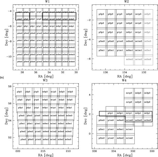
Layout of the four CFHTLenS patches. The grey pointings in the W2 region denote fields with incomplete colour coverage. They are not included in the CFHTLenS project. Enclosed areas in W1 and W4 indicate regions of available spectroscopic redshifts for a photometry crosscheck as discussed in Section 5.1. See the text for further details.
Table 1 contains observational details and provides average quality characteristics of our co-added CFHTLenS pointings. It lists the targeted observing time for the different filters, the mean limiting magnitudes and the mean seeing values with their corresponding standard deviations over all CFHTLenS pointings. The seeing is estimated using the SExtractor (see Bertin & Arnouts 1996)3 parameter FWHM_IMAGE for stellar sources. Our limiting magnitude, mlim, is the 5σ detection limit in a 2.0 arcsec aperture.4 Nearly all 171 pointings in all filters were obtained under superb, photometrically homogeneous and sub-arcsecond seeing conditions (see also Table A1). In Fig. 2, we show the full seeing distribution for all fields and filters. It does not show the skewness to large values that is typical in large and long-term observing campaigns without imposed seeing constraints.
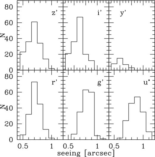
Seeing distributions for all CFHTLenS fields and filters.
Characteristics of the final CFHTLenS co-added science data (see the text for an explanation of the columns).
| Filter | Expos. time (s) | mlim (AB mag) | Seeing (arcsec) |
|---|---|---|---|
| 5σ lim. mag. | |||
| in a 2.0 arcsec aperture | |||
| u*(u.MP9301) | 5 × 600 (3000) | 25.24 ± 0.17 | 0.88 ± 0.11 |
| g′(g.MP9401) | 5 × 500 (2500) | 25.58 ± 0.15 | 0.82 ± 0.10 |
| r′(r.MP9601) | 4 × 500 (2000) | 24.88 ± 0.16 | 0.72 ± 0.09 |
| i′(i.MP9701) | 7 × 615 (4305) | 24.54 ± 0.19 | 0.68 ± 0.11 |
| y′(i.MP9702) | 7 × 615 (4305) | 24.71 ± 0.13 | 0.62 ± 0.09 |
| z′(z.MP9801) | 6 × 600 (3600) | 23.46 ± 0.20 | 0.70 ± 0.12 |
We note that the original CFHT i′-band filter (CFHT identification: i.MP9701) broke in 2008 and a total of 33 fields were obtained with its successor (CFHT identification: i.MP9702). 19 fields, whose point spread function (PSF) properties in the original i′-band observations were classified as problematic for weak lensing studies, have observations in both filters. If necessary, we distinguish the two with labels i′ for i.MP9701 and y′ for i.MP9702. A table detailing important quality properties for each pointing and filter is given in Appendix A.
3 DATA PROCESSING
The primary goal of the image processing modules we created is to provide the following products, necessary for the weak lensing and photometric redshift analyses.
Deep, co-added astrometrically and photometrically calibrated images for all CFHTLenS pointings in each filter. These images are primarily used to define the source catalogue sample for our lensing studies and to estimate photometric redshifts; see Hildebrandt et al. (2012). A short summary can be found in Appendix C. Each co-added science image is accompanied by an inverse-variance weight map which describes its noise properties (see e.g. fig. 2 of Erben et al. 2009). In addition, we create a so-called sum image. This is an integer-value image which gives, for each pixel of the co-added science image, the number of single frames that contribute to that pixel. It is used to easily identify image regions that do not reach the full survey depth, such as areas around chip or edge boundaries.
For the i′-filter observations, which are used for our shape and lensing analysis, we require sky-subtracted individual chips that are not co-added. They are accompanied by bad-pixel maps, cosmic ray masks, and precise information of astrometric distortions and photometric properties. In connection with the object catalogues extracted from the co-added images, these products are primarily used by our lensfit weak shear measurement pipeline. The procedures to model the PSF and to determine object shapes on the basis of individual exposures are described in detail in Miller et al. (2013). The quality of the shear estimates is discussed in Heymans et al. (2012).
Each CFHTLenS science image is supplemented by a mask, indicating regions within which accurate photometry/shape measurements of faint sources cannot be performed, e.g. due to extended haloes from bright stars.
The methods and algorithms used to obtain the imaging products are heavily based on our developments within the CFHTLS Archive Research Survey (CARS) project (see Erben et al. 2009). In the following, we give a thorough description of the steps that contain significant changes and improvements. The main differences concern data treatment on the patch level within CFHTLenS; while for CARS we treated each survey pointing independently, we now simultaneously treat all images within a patch. This optimally utilizes available information to obtain a homogeneous astrometric and photometric calibration over the patch area. Our data processing is described in the following.
3.1 Data retrieval from CADC
We start our analysis with the elixir5 preprocessed CFHTLS-Wide data available at the Canadian Astronomical Data Centre (CADC).6 Exposure lists for the CFHTLS surveys can be obtained from CFHT.7 Besides the primary CFHTLS-Wide imaging data, the catalogue lists, for each patch, exposures of an astrometric presurvey. This presurvey densely (re)covers the complete patch area with short (180 s) r′-band exposures. The footprint for the presurvey fields is different from the science pointings to enable a good mapping of camera distortions. A single exposure was obtained at each presurvey position. At the end of the survey, each patch was similarly complemented with additional exposures obtained under photometric conditions in all filters. Each of these photometric pegs overlaps with four science pointings and helps to ensure a homogeneous photometric calibration on the patch level. Fig. 3 outlines the available data for patch W4. The photometric pegs were not obtained under the primary CFHTLS programme but under the CFHT programme IDs 08AL99 and 08BL99. Using the relevant exposure IDs, all data were retrieved from CADC. Besides the image list, the CFHTLS exposure catalogue also contains information on the conditions of the observations. Only data that are marked as either completely within survey specifications or as having one of the predefined specifications (seeing, sky transparency or moon phase) slightly out of bounds8 enter the following process. We note that the availability of this quality information made laborious quality checks on each image unnecessary at this stage.
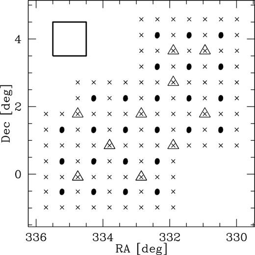
Available data in the W4 patch area: the dots denote the centres of primary science observations, the crosses indicate the centres of exposures of the astrometric presurvey and the triangles mark the centres of additional photometric pegs. The square in the upper-left corner shows the MegaPrime field of view.
3.2 Processing of single exposures
In addition to raw data, CADC offers all CFHTLS images in elixir preprocessed form. The elixir processing (see Magnier & Cuillandre 2004) includes removal of instrumental signatures. This spans overscan and bias subtraction, flat-fielding, removal of fringing in i′ and z′, and photometric flattening across the MegaPrime field of view. In addition, each exposure comes with photometric calibration information (zero-point, extinction coefficient and colour term).9
Starting from the elixir images, we perform the following processing steps (see Erben et al. 2009 for more details).
We identify and mark individual exposure chips that should not be considered any further using a Flexible Image Transport System (FITS) header keyword. This concerns chips that either contain no information (all pixel values equal to zero) or where more than 5 per cent of the pixels are saturated. In the latter case, ghosts from very bright stars render most of the chip data unusable. In contrast to CARS, we do not automatically mark chips in other colours of a pointing as bad if the corresponding i′-band chip is flagged.
We create sky-subtracted versions of all chips with SExtractor.
We create a weight image for each science chip as outlined in Erben et al. (2005) and as detailed for MegaPrime data in section A.2 of Erben et al. (2009). As described in these publications, we aim for a complete identification of image artefacts on the level of individual chips to perform a weighted-mean co-addition of the data later on. Cosmic rays in our data are detected with a neural network algorithm that utilizes SExtractor with a special cosmic ray filter. This filter is constructed with the eye program10(see Bertin 2001). In the course of our analysis, we noted a significant confusion of stellar sources with cosmic rays in images obtained under superb seeing conditions. The effect is highly notable for a seeing below ∼0.6 arcsec. In Section 4, we describe in detail how this confusion is treated.
Utilizing the weight image we extract reliable, high-S/N object catalogues from each chip (SExtractor DETECTION_MINAREA/DETECTION_THRESH is set to 5/5 for g′r′i′y′z′ and to 3/3 for u*), which are used for our astrometric and photometric calibration.
Finally, we study the PSF properties of each chip by analysing bright, unsaturated stars with the Kaiser–Squires–Broadhurst (KSB) algorithm (see Kaiser, Squires & Broadhurst 1995). This is done primarily to reject images with badly behaved PSF properties such as a large stellar ellipticity at a later stage; see Section 3.3.
3.3 Astrometric and photometric calibration
The most significant difference between the CARS and the CFHTLenS data processing concerns the astrometric and photometric calibration. While we treated each pointing separately and independently in CARS, we now perform these calibration steps simultaneously for all exposures of a patch within CFHTLenS. By treating all available data at the same time, we expect an increased homogeneity in the astrometric and photometric properties of the data. The main pillar of this processing unit is the scamp program in version 1.4.611 (see Bertin 2006), which is specifically designed for accurate astrometric and photometric calibration of large imaging surveys. The size of the survey that can be calibrated with scamp in a single step is only limited by computational resources, especially the main memory. We perform the following calibration steps.
Our astrometric reference catalogues are 2MASS (see Skrutskie et al. 2006) for W1, W2 and W4 and SDSS-DR7 (see Abazajian et al. 2009) for W3. Unfortunately, the SDSS-DR7 only covered patch W3 completely and small parts of the other CFHTLenS areas. We note that for SDSS-DR7, we only used sources with iSDSS < 18 for our calibrations. For the following astrometric calibration process which is based on associating source lists from our single-frame images and the standard star catalogue, it is favourable if both samples have approximately the same density. Objects which are only present in one catalogue decrease the source matching contrast and do not add anything to constrain the solution. This is the case for the fainter SDSS sources which have no counterpart in our single-frame source samples. In contrast, the intrinsic depth of 2MASS very well matches single-frame sources obtained with our extraction parameters; see Section 3.2.
The available computer equipment12 allowed us to calibrate all exposures (primary science, astrometric presurvey, photometric pegs) from all filters of the smaller patches W2 and W4 simultaneously. Both patches consist of about 1000 individual MegaPrime exposures with 36 chips each. The larger patches W1 (∼3000 exposures) and W3 (∼2000 exposures) had to be split for our scamp runs. First, we separately process the r′ filter, which consists of science data in addition to the astrometric presurvey images. Next, the remaining filters u*, g′, i′ and z′ were individually calibrated together with the r′ band, so that each filter profited from the astrometric presurvey information. In addition to astrometric calibration, scamp uses sources from overlapping exposures to perform a relative photometric calibration. For each exposure, i, of a specific filter, f, we obtain a relative magnitude zero-point, ZPrel(i, f), giving us the magnitude offset of that image with respect to the mean relative zero-point of all images. That is, we demand ∑iZPrel(i, f) = 0. Note that this procedure calibrates data obtained under photometric and non-photometric conditions on a relative scale. An absolute flux scaling for the patch can be obtained from the photometric subset; see below.13
After the first scamp run, we reject exposures suffering from an atmospheric extinction larger than 0.2 mag. We also remove images showing a large PSF ellipticity over the field of view. Large, homogeneous PSF anisotropies are mostly a sign of tracking problems during the exposure. All images that have a mean stellar ellipticity (the mean is taken over all chips of the image and it is estimated with the KSB algorithm) of 0.15 or larger are discarded from further analyses. Utilizing the remaining images, we perform another scamp run to conclude the astrometric and relative photometric calibration of our data. For each patch and filter, we manually verify the distributions of typical quality parameters (sky-background level, seeing, stellar ellipticity, relative photometric zero-point). None of the plots showed suspicious images that should be removed at this stage. See Fig. 4 for an example of our patch-wide check plots.
- The last step of the astrometric and photometric calibration is the determination of the absolute photometric zero-point on the patch level. Input to our procedure are the relative zero-points from scamp, photometric zero-points and extinction coefficients from elixir, and the list of exposures that were obtained under photometric conditions. Information on the sky transparency of each image is included in the CFHTLS exposure catalogue (see Section 3.1). For all photometric exposures, i, in a filter, f, from a given patch, we calculate a corrected zero-point, ZPcorr(i, f), according towhere ZP(i, f) is the instrumental AB zero-point, AM(i, f) is the airmass during observation and EXT(i, f) is the colour-dependent extinction coefficient. For photometric data, the relative zero-points compensate for atmospheric extinction and the corrected zero-points agree within measurement errors. We iteratively estimate the mean ZP(f) = 〈ZPcorr(f)〉i of all exposures, i, by rejecting 3σ outliers. We stop iterating once no more data are rejected. With more than 100 exposures marked as photometric in each patch and filter, this procedure ensures a robust estimation of the patch zero-point. Our iterative procedure to estimate 〈ZPcorr(f)〉i typically rejected less than 5 per cent of the data that are initially marked as photometric by elixir. Only in four cases (W1 u*, W1 g′, W1 i′ and W2 g′) the rejection rate was about 10 per cent. This confirms that the photometric calibration from CFHT is very good. The final ZP(f) is used as the absolute magnitude zero-point for all co-added images of filter, f, in a particular patch.\begin{equation*} {\rm ZP}_{{\rm corr}}(i, f) = {\rm ZP}(i, f) + {\rm AM}(i, f) {\rm EXT}(i, f) + {\rm ZP}_{{\rm rel}}(i, f), \end{equation*}
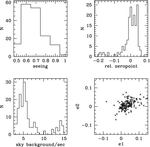
Quality parameter distributions of all 164 W4 i′-band exposures that enter the co-addition and science analysis stage. Shown are the seeing distribution (top left), the distribution of relative photometric zero-points as determined by scamp (top right), the sky-background brightness in ADU s−1 (bottom left) and the two components of stellar PSF ellipticities (bottom right). All quantities are estimated as mean values over all 36 chips of a specific exposure. See the text for further details.
We assess the quality of our astrometric and photometric calibration in Section 5.
3.4 Image co-addition and mask creation
In the subsequent analysis, co-added data are used in the detection of stars and galaxies and in the photometric measurements and analysis (Hildebrandt et al. 2012). Co-added data are not used for the lensing shear measurement (Miller et al. 2013). One of our main goals for the co-added images is to ensure data with homogeneous image quality. We therefore check for each pointing/filter combination whether the exposure set consists of images with large seeing variations. For instance, our best seeing pointing W4m3p1 i′ band has a co-added image seeing of 0.44 arcsec though originally it has four individual exposures with image qualities of 0.43, 0.47, 0.48 and 0.88 arcsec. To avoid degradation of the superb quality images below 0.5 arcsec with the image of 0.88 arcsec, we want to reject the last image from the co-addition process. We estimate the median (med) of the seeing values of a pointing/filter combination and reject data that have a larger seeing than med + 0.25. In addition, for the i′-band data, which form the basis for our source catalogues, images with a seeing larger than 1.0 arcsec are not included in the co-addition process. Note that our procedure ensures homogeneity on the pointing/filter level and avoids rejection of data with fixed quality values on the patch level.14
Finally, the sky-subtracted exposures belonging to a pointing/filter combination are co-added with the swarp program (version 1.38)15 (see Bertin et al. 2002). We use the LANCZOS3 kernel to remap original image pixels according to our astrometric solutions. The subsequent co-addition is done with a statistically optimally weighted mean which takes into account sky-background noise, weight maps and the relative photometric zero-points as described in section 7 of Erben et al. (2005). As sky projection we use the TAN projection (see Greisen & Calabretta 2002). The reference points of the TAN projection for each pointing are those defined for the CFHTLS-Wide survey.16 After co-addition we extend all images with blank borders to a common size of 21 k × 21 k pixels around the image centre. This comprises areas with useful data for all CFHTLenS pointings. The image extension is necessary because our later multicolour analysis of CFHTLenS pointings with the SExtractor dual-image mode requires pixel data of equal dimensions. The swarp information and photometric zero-points are also passed to the lensing shear analysis of the individual exposures, although a key part of the shear measurement is that the data are not interpolated on to a new reference frame when measuring galaxy shapes (Miller et al. 2013).
As a final step, we use the automask tool17 (see Dietrich et al. 2007) to create image masks for all pointings. These masking procedures are described in detail in Erben et al. (2009). Within CFHTLenS all 171 automatically generated masks are manually double-checked and, if necessary, refined. We note that the lensing catalogue quality assessment performed in Heymans et al. (2012) shows that lensing analyses with the automatic masks and the refined versions are consistent.
The result of this step is co-added science images for all 171 CFHTLenS pointings in all filters. Each science image is accompanied by a weight and a sum image as described in Section 3. These products, together with the sky-subtracted individual chip data and the astrometric information from scamp (see Section 3.3), form the basis for all CFHTLenS shear and photometric analyses.
4 INFLUENCE OF OUR COSMIC RAY REMOVAL ON STELLAR SOURCES
As discussed in Section 3.2, our procedure to identify cosmic rays in individual MegaPrime exposures is based on a neural network approach. During the weak lensing analysis with lensfit, we noticed that a large number of individual exposures had very few stars suitable for a PSF analysis. We traced the problem to the cores of point sources being misclassified and masked as cosmic rays. A closer analysis revealed that the problem was worst for the best seeing exposures, and the neural network approach is the primary source of the problem. In the following, our main goal is to unflag bright, unsaturated stars suitable for PSF analyses with lensfit and PSF homogenization within our photometric redshift (photo-z) analyses (see Hildebrandt et al. 2012). We explicitly note that we did not aim for a complete solution to the problem within CFHTLenS. Our prescription to identify and to unflag bright stars after the initial cosmic ray analysis is as follows. (1) We run SExtractor on individual exposure chips with a high detection threshold (DETECTION_MINAREA/DETECTION_THRESH is set to 10/10). This SExtractor run is performed without using weighting or flagging information. (2) Candidate stellar sources are identified on the stellar locus in the size–magnitude plane. (3) We perform a standard PSF analysis with the KSB algorithm. This involves estimating weighted second-order brightness moments for all candidate stars and to perform, on the chip level, a two-dimensional second-order polynomial fit to the PSF anisotropy. The fit is done iteratively with outliers removed to obtain a clean sample of bright, unsaturated stars suitable for a PSF analysis. (4) We remove cosmic ray masks in a square of 4 × 4 pixels around stellar sources that are still included in our sample after step (3). Fig. 5 shows the result of our analysis on pointing W1m2m1 in the i′ band. The set consists of seven exposures with an image quality between 0.48 and 0.55 arcsec, including five images below 0.5 arcsec. The figure also shows the stellar locus of the co-added image before (left-hand panel) and after (right-hand panel) we modified the cosmic ray masks of individual exposures. We note that our procedure returns a significant number of stars to the sample. In the corrected version we also see an abrupt break in the stellar locus at i′ ≈ 22. For our i′-band data, this marks the limit to identify usable stars for PSF studies with our KSB approach, and we would need another procedure to also reliably identify fainter stars that are confused as cosmic rays. We would like to reiterate that our main goal within CFHTLenS is to have a sufficient number of bright, unsaturated stars for a reliable PSF analysis with lensfit, but none of our science projects requires complete and unbiased stellar samples down to faint magnitudes. We identified the stellar break problem to be immediately noticeable in images with a seeing of about 0.6 arcsec and better. The better the image quality, the more prominent is this feature. In the co-added images with an overall seeing of 0.7–0.75 arcsec, we can still identify stellar breaks if the set contains exposures in the best seeing range. In Fig. 6, we show prominent stellar breaks for i′ ≈ 22, z′ ≈ 21, r′ ≈ 22.5 and g′ ≈ 23.
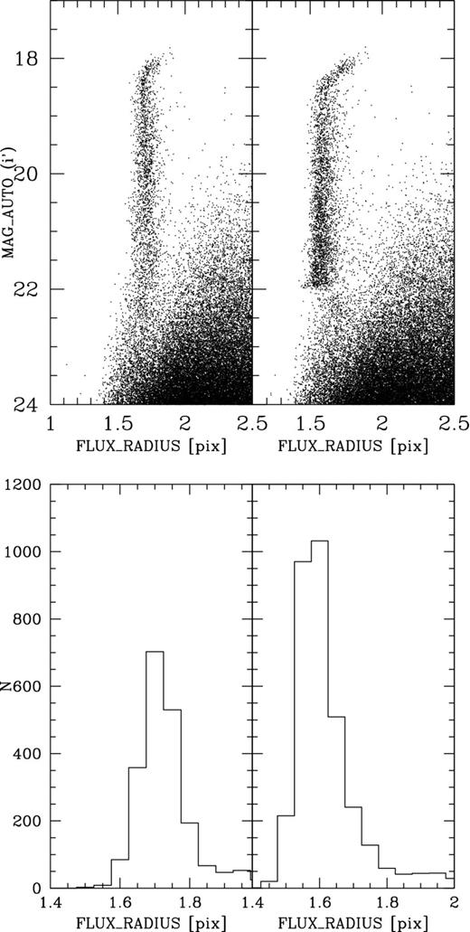
Stellar break in the co-added image of W1m2m1 i′ band, with a seeing of 0.47 arcsec. Shown are stellar loci in the size–mag plane (SExtractor quantities FLUX_RADIUS and MAG_AUTO; top panels). The top-left panel shows the stellar locus after our standard cosmic ray removal procedure, the top-right panel after we bring back stars whose cores were falsely classified as cosmic rays. The lower panels show corresponding histograms of object counts for |$1.4<{\tt {FLUX\_RADIUS}}<2.0$| and i′ < 22.0. See the text for further details.
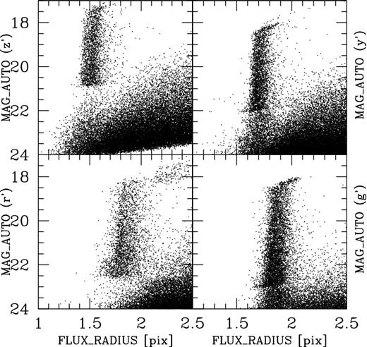
Stellar break in W1p4p1 z′ band (0.46 arcsec, top left), W3m2m1 y′ band (0.51 arcsec, top right), W1p4p1 r′ band (0.52 arcsec, bottom left) and W4p1p1 g′ band (0.58 arcsec, bottom right); see the text for further details.
We do not observe obvious breaks in the loci of u*, where the best quality co-added image has an image seeing of 0.62 arcsec, and only some in g′. Fields with obvious stellar breaks are indicated in the comments column of Table A1. The judgement was done subjectively by manually checking stellar locus plots from all 171 CFHTLenS pointings. We specifically note that our cosmic ray removal procedure did not influence the detection nor the photometry of galaxies.
5 EVALUATION OF ASTROMETRIC AND PHOTOMETRIC PROPERTIES
Our data underwent substantial testing and quality control for our main scientific objective: weak gravitational lensing studies with photometric redshifts for all galaxies. The quality of our lensfit shear estimates and the accuracy of photometric redshifts are described in detail in Heymans et al. (2012) and Hildebrandt et al. (2012). These analyses have demonstrated the robustness of our data set. Here we mainly quote the precision we were able to achieve in our astrometric and photometric calibration.
To quantify our astrometric accuracy with respect to external sources, we compare object positions in our CFHTLenS pointings with the SDSS-DR9 catalogue (see Ahn et al. 2012). Note that SDSS-DR918 was not used as an external astrometric catalogue for our astrometric calibration. It only became available after our data processing was completed. It is, after SDSS-DR8, the second SDSS catalogue that covers all but 10 CFHTLenS pointings. The fields without SDSS-DR9 overlap are W1p3m4, W1p4m4 and the 10W2 pointings south of −4° in declination (see Fig. 1). Fig. 7 summarizes our astrometric accuracy compared to the SDSS reference. We compare the position of SDSS stellar sources with iSDSS < 21 to each pointing and filter. Object positions in our data were estimated independently for each filter in the corresponding co-added images. The star classification was taken from the SDSS catalogue. Fig. 7 shows the mean deviation (the mean is taken over all sources in all filters in a patch) of positions and the standard deviation of the positional differences. We see that the CFHTLenS data show a systematic offset in right ascension and declination of less than 0.2 arcsec in all cases. The standard deviation is uniform over all fields and its distribution peaks at about 50–70 mas for all CFHTLenS patches. If we assume that the SDSS astrometry is superior to that of 2MASS, Fig. 7 gives us a good indication on the absolute accuracy of 2MASS within CFHTLenS patches W1, W2 and W4. As discussed in Section 3.3, the higher intrinsic depth of an SDSS catalogue with respect to 2MASS does not help to constrain an astrometric solution with our setup. Therefore, the main advantage of SDSS compared to 2MASS is its increased absolute astrometric accuracy.
Astrometric comparison with SDSS-DR9. Shown are object position comparisons between CFHTLenS sources in all pointings for the i′ filter with SDSS iSloan < 21 stars. The solid, dotted, short-dashed and long-dashed histograms show comparisons of W1, W2, W3 and W4, respectively. See the text for further details.
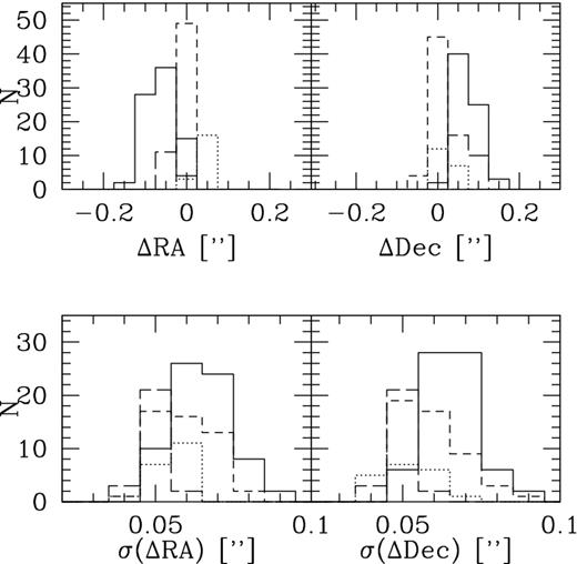
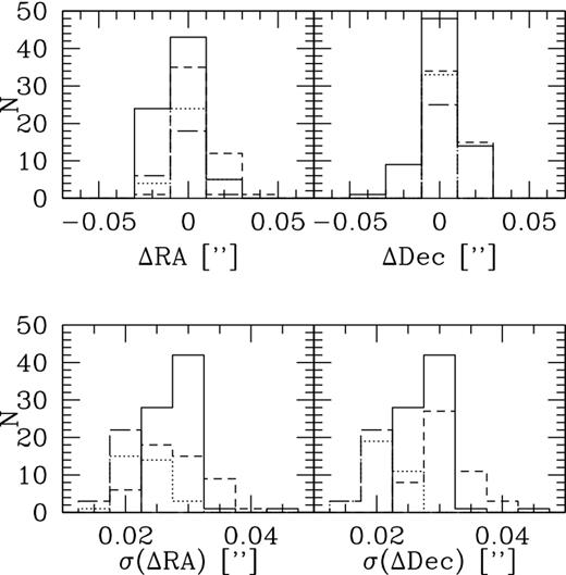
In Figs 8 and 9, we quantify the internal astrometric accuracy, comparing positions of sources observed in different filters of all pointings. We use objects with |$i^{\prime }_{{\rm {CFHTLenS}}} < 21$| that are classified as stars by SExtractor (CLASS_STAR > 0.95). The sources were extracted from the co-added images. Fig. 8 shows positional differences within individual CFHTLenS pointings. We see that we cannot detect significant systematic offsets in right ascension and declination between the colours. The rms positional difference between the filters is about 30 mas. In Fig. 9 we show positional differences with sources on different CFHTLenS pointings. As before, we match objects regardless of their filter, but only allow associations from different, adjacent CFHTLenS pointings. We only show the W1 comparison here – results are similar for the other patches. The error parameters are comparable to the interpointing comparison. Absolute positional differences are evenly distributed around zero and the rms deviations are σ(ΔRA) = 0.030 arcsec and σ(ΔDec.) = 0.027 arcsec.
Internal astrometric accuracy. Shown are internal astrometric positional differences between the different filters within individual CFHTLenS pointings. The solid, dotted, short-dashed and long-dashed histograms show comparisons of W1, W2, W3 and W4, respectively. See the text for further details.
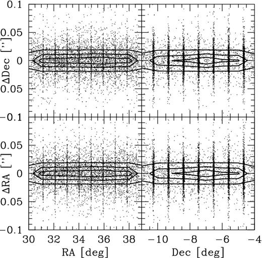
Internal astrometric accuracy on overlap sources in W1. We show positional differences between object matches of CFHTLenS sources in different, adjacent pointings. The comparison is done in W1 across all filters. The vertical stripes in the density distribution originate from the alignment of overlap regions; see Fig. 1. The contours indicate areas of 0.7, 0.4 and 0.05 times the peak value of the point-density distribution. For clarity of the plot, only 1 point out of 100 is visualized. See the text for further details.
The photometric calibration of CFHTLenS is also evaluated by direct comparison to SDSS-DR9. The availability of SDSS data nearly overlapping the full CFHTLenS area allows us to obtain a comprehensive understanding of the photometric quality of our data. We would like to reiterate that the SDSS data were not used at any stage of the data calibration phase.
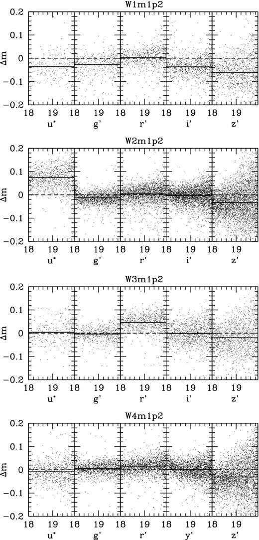
Magnitude comparisons between SDSS stars with and CFHTLenS sources for the fields W1m1p2 with x ∈ {1, 2, 3, 4}. The solid horizontal lines indicate |$\langle \Delta {\textit {m}}\rangle$|. The precise values of the mean offsets and formal standard deviations can be found in Table A1. Note that W4 and W2 are at significantly lower galactic latitude than W1 and W3; thus, the stellar density in the latter two is substantially lower.
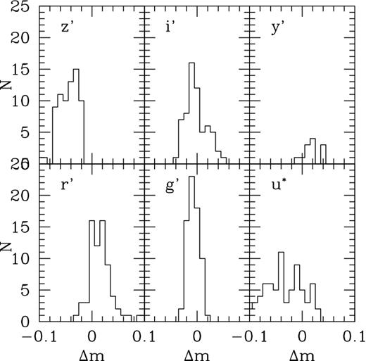
Distribution of the differences between SDSS and CFHTLenS magnitudes in W1. The abscissa of the plots shows Δm = mCFHTLenS − mSDSS. See the text for further details.
Given the results from the SDSS-DR9 comparison, we summarize accuracies for the individual patches and filters in Table 2. We quote the mean of all average deviations in the individual pointings and their corresponding standard deviations. The values indicate that we obtain on average a homogeneous calibration of our data. This result is confirmed by the quality of our photometric redshifts presented in Hildebrandt et al. (2012). Since then we were able to further test our photo-z estimates with new spectroscopic redshifts on a significant part of the CFHTLenS area. This additional confirmation for the robustness of our photometry is described in the next section.
Average photometric accuracies in the CFHTLenS patches.
| Patch | Filter | Phot. accuracy | Patch | Filter | Phot. accuracy |
|---|---|---|---|---|---|
| W1 | u* | −0.034 ± 0.035 | W1 | i′ | −0.002 ± 0.020 |
| W2 | u* | +0.034 ± 0.031 | W2 | i′ | −0.009 ± 0.020 |
| W3 | u* | −0.045 ± 0.043 | W3 | i′ | +0.003 ± 0.015 |
| W4 | u* | −0.001 ± 0.014 | W4 | i′ | −0.003 ± 0.021 |
| W1 | g′ | −0.007 ± 0.011 | W1 | y′ | +0.019 ± 0.015 |
| W2 | g′ | +0.004 ± 0.013 | W2 | y′ | +0.022 ± 0.022 |
| W3 | g′ | −0.007 ± 0.012 | W3 | y′ | −0.001 ± 0.022 |
| W4 | g′ | −0.002 ± 0.010 | W4 | y′ | +0.022 ± 0.050 |
| W1 | r′ | +0.017 ± 0.024 | W1 | z′ | −0.045 ± 0.018 |
| W2 | r′ | +0.014 ± 0.012 | W2 | z′ | −0.054 ± 0.012 |
| W3 | r′ | +0.022 ± 0.014 | W3 | z′ | −0.036 ± 0.016 |
| W4 | r′ | +0.014 ± 0.006 | W4 | z′ | −0.030 ± 0.017 |
5.1 Comparison of CFHTLenS photo-z with spectroscopic redshifts
The derivation of the CFHTLenS photo-z is detailed in Hildebrandt et al. (2012), where we compared the photo-z to spectroscopic redshifts (spec-z) from VIMOS VLT Deep Survey (VVDS; Le Fèvre et al. 2005), DEEP2 (Davis et al. 2007) and SDSS-DR7 on 20 of the 171 CFHTLenS fields. More spec-z have since become available through the Visible Multi-Object Spectrograph Public Extragalactic Redshift Survey (VIPERS; see Guzzo et al., in preparation).22 In this paper, we study how the CFHTLenS photo-z compare to VIPERS on 22 additional fields independent from the 20 fields tested in Hildebrandt et al. (2012).
Fig. 12 shows a direct comparison of the CFHTLenS photo-z versus VIPERS spec-z of 18 995 objects. Note that the VIPERS spec-z catalogue is pre-selected by colour, targeting mostly objects in the range 0.5 ≲ z ≲ 1.2 down to i′ ≈ 22.5. We estimate photo-z statistics (scatter, outlier rate, bias and completeness) as a function of i′-band magnitude and redshift in the same way as described in Hildebrandt et al. (2012). The results are shown in Figs 13 and 14. Comparing to the performance of the CFHTLenS photo-z versus VVDS/DEEP2/SDSS spec-z, we do not find any significant differences in the magnitude range (i′ ≲ 22.5) and redshift range (0.5 ≲ z ≲ 1.2), where VIPERS spec-z are available.
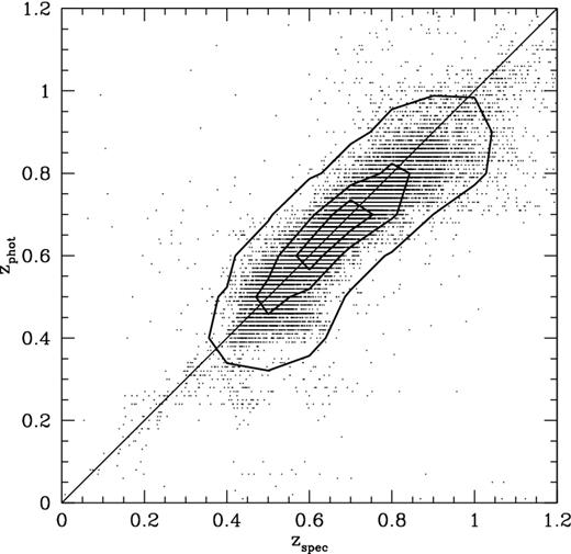
Photo-z versus spec-z for the 22 CFHTLenS fields with VIPERS overlap. Shown are all objects with secure spec-z. No magnitude cut is applied. The contours indicate regions around 0.7, 0.4 and 0.05 times the peak value of the point-density distribution.
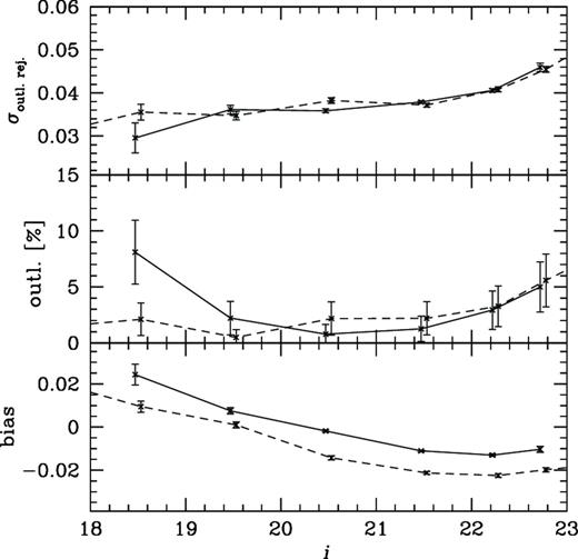
Photo-z statistics as a function of magnitude. The top panel shows the photo-z scatter after outliers were rejected, the middle panel shows the outlier rate and the bottom panel shows the bias (outliers included; positive means photo-z's overestimate the spec-z's). Errors are purely Poissonian. Note that the errors between magnitude bins are correlated. The solid curve shows statistics for the analysis of this paper. For comparison, we also show corresponding measurement from Hildebrandt et al. (2012) (dashed curve).
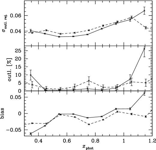
Similar to Fig. 13 but here statistics are a function of photo-z. We only plot the redshift interval where VIPERS yields a sufficient number of spec-z. The solid curve shows statistics for the analysis of this paper. For comparison, we also show the corresponding measurement from Hildebrandt et al. (2012) (dashed curve).
This test suggests that the photo-z accuracy (and hence also the photometry) is stable over the survey area, beyond the fields that could be tested with the original spec-z catalogues. Having such a successful blind test – a posteriori – is a strong argument for the stability of our global photometry, and confirms that the photo-z statistics presented in Hildebrandt et al. (2012) can be assumed for the whole survey with a greater degree of confidence.
5.2 Galaxy correlation functions on large angular scales
As a further test for the photometric homogeneity of our data beyond individual pointings, we investigate the galaxy correlation function out to large angular scales. The behaviour of the large-scale galaxy angular correlation function, w(θ), is a sensitive diagnostic test of large-scale systematic photometric gradients in an imaging data set. Such photometric gradients would cause systematic density variations in a source sample selected above a given flux threshold. Our correlation analysis compares the actual galaxy positions against a randomly generated, uniformly distributed source distribution. Hereby, the random catalogue precisely follows the geometry that is available to objects in the data, i.e. taking into account our image masks. Therefore, any photometric gradient will result in an excess of signal in the large-scale w(θ) such that it does not asymptote to zero. In contrast to the tests described above, we here use our patch-wide science object catalogues described in Hildebrandt et al. (2012) and Appendix C. We use all galaxies down to i′ = 22, which results in the following sample sizes: 656 998 galaxies in W1, 217 359 in W2, 483 333 in W3 and 189 209 in W4. The random comparison catalogues in each patch have four times the corresponding object count.
We measure w(θ) for all four CFHTLenS regions in 30 logarithmic angular bins between 0|${^{\circ}_{.}}$|003 and 3° with the Landy & Szalay (1993) estimator. We restrict the sample to objects with star–galaxy classifier |${\tt {star\_flag}} = 0$| and |${\tt {MASK}} = 0$| (see Appendix C), and consider three magnitude thresholds i′ < (20, 21, 22). The integral constraint correction is applied to the correlation functions. We determine the errors in the measurement using jack-knife re-sampling. The jack-knife samples are extended across all four regions such that each sample has a characteristic size of 3°; 54 jack-knife samples are used in total. We note that the measurements in the different CFHTLenS regions produce consistent results within the expectation of cosmic variance, with the dispersion between the regions becoming minuscule at small angular scales.
The combined correlation function measurements of the four patches are plotted in Fig. 15 and compared to the predictions of a Λ cold dark matter cosmological model following Smith et al. (2003). This prediction is generated from a camb (see Lewis, Challinor & Lasenby 2000) + halofit non-linear power spectrum (produced using cosmological parameters consistent with the latest CMB measurements), combined with galaxy redshift distributions produced by stacking the photometric redshift probability distributions at each magnitude threshold, and assuming a linear galaxy bias factor b ∼ 1.2. The measurements are consistent with the model at large scales, and tend to zero there, revealing no evidence for systematic photometric gradients in the sample. The model is not expected to be a good match to the data at scales below |$1\,{Mpc}\,h_{72}^{-1}$|,23 where non-linear and halo model effects become important.
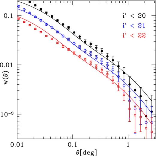
Combined angular galaxy correlation functions for CFHTLenS patches W1 to W4. The solid lines show theoretical predictions; see the text for further details.
We stress that we present this analysis primarily to further strengthen confidence in the integrity of our photometric catalogues. We do not want to present an in-depth investigation of the angular galaxy correlation function or to interpret it scientifically. This will be done in Bonnett et al. (in preparation).
6 RELEASED DATA PRODUCTS
In the spirit of the CFHTLS, we make all data used for scientific exploitation by the CFHTLenS team available to the astronomical community. The released data package includes the following.
The co-added CFHTLenS pixel data products consisting of primary science data, weight and flag maps, sum frames and image masks. All these products are introduced and described in Section 3.4. Important details for potential users are provided in Appendix B.
The CFHTLenS source catalogues with all relevant photo-z and lensing/shear quantities. The creation of these catalogues is described in Hildebrandt et al. (2012) and Miller et al. (2013). The catalogue entries are described in Appendix C.
The data are made available by CADC through a web interface and can be found at http://www.cadc-ccda.hia-iha.nrc-cnrc.gc.ca/community/CFHTLens/query.html. The interface allows users to retrieve image pixel data on a pointing/filter basis. The catalogues can be accessed with a sky-coordinate query form with filter options on all catalogue entries.
7 CONCLUSIONS
We have presented the CFHTLenS data products that originate from the CFHTLS-Wide survey. CFHTLS-Wide was specifically designed as a weak lensing survey providing deep, high-quality optical data in five passbands. Prior to the scientific exploitation of the data, the CFHTLenS collaboration had the objective to develop and to thoroughly verify all necessary algorithms and tools in order to fully exploit the survey. This development includes numerous refinements to existing data processing techniques, in particular an optimal treatment in the astrometric and photometric calibration phase. Another important upgrade of our analysis was to develop an algorithm to nearly automatically perform the important image masking task. Hitherto, it has mainly been performed manually. It is important to stress that specific, high-precision scientific applications such as our weak lensing analyses generally require very specific data processing steps. These often tend to be in conflict with a general-purpose data set which needs to fulfil the requirements of diverse scientific applications. Where necessary, our data processing was heavily specialized to analyse small and faint background sources that are essential for all weak lensing studies. This affects for instance our sky-background subtraction which aims for a local sky background as flat as possible on small angular scales. Furthermore, our treatment of cosmic rays has been optimized for a robust identification of cosmic ray hits on the basis of individual images. This was crucial for the lensfit shear pipeline which entirely operates on single frames instead of the co-added images. As described in Section 4, our current implementation leads to a strong incompleteness of stellar counts at faint magnitudes. For this reason, the CFHTLenS data are complementary to other publicly released versions of the CFHTLS-Wide survey.24
We have demonstrated that we are able to produce a homogeneous and high-quality data set suitable for weak lensing studies with photometric redshift estimates. Our external astrometric accuracy with respect to SDSS data is around 60–70 mas, and the internal alignment in all filters is around 30 mas. Our average photometric calibration shows a dispersion with respect to SDSS of the order of 0.01–0.03 mag for g′, r′, i′ and z′ and about 0.04 mag for u*. We show in Heymans et al. (2012), Miller et al. (2013) and Hildebrandt et al. (2012) that our data have the necessary quality to fully exploit the scientific potential of a 154 deg2 weak lensing survey.
The newly available SDSS-DR9 data, covering almost the complete CFHTLenS area, will allow us to further refine our algorithms and procedures in the future, especially increasing the quality of our photometry. This will be particularly useful in preparation for the next generation of weak lensing surveys that will cover substantial parts of the sky, such as the 1500 deg2 Kilo-Degree Survey25 (de Jong et al. 2012) or the 5000 deg2 Dark Energy Survey26 (Mohr et al. 2012). For these surveys, the accuracy of current algorithms certainly needs to be further improved to exploit their full scientific potential and to be not dominated by residual systematics.
In the hope that we will trigger a variety of new developments and follow-up studies with the CFHTLenS products, we make the complete data set, consisting of pixel data and object catalogues with all relevant lensing and photo-z quantities, publicly available via CADC.
We thank the VIPERS collaboration, for a fruitful data exchange and for providing us with unpublished spectroscopic redshifts. We also thank TERAPIX for the individual exposure quality assessment and validation during the CFHTLS data acquisition period, and Emmanuel Bertin for developing key software modules used in this study. CFHTLenS data processing was made possible thanks to significant computing support from the NSERC Research Tools and Instruments grant programme. We thank the CFHT staff for successfully conducting the CFHTLS observations and in particular Jean-Charles Cuillandre and Eugene Magnier for the continuous improvement of the instrument calibration and the elixir detrended data that we used.
This work is based on observations obtained with MegaPrime/MegaCam, a joint project of CFHT and CEA/DAPNIA, at the Canada–France–Hawaii Telescope (CFHT) which is operated by the National Research Council (NRC) of Canada, the Institut National des Sciences de l’Univers of the Centre National de la Recherche Scientifique (CNRS) of France and the University of Hawaii. This research used the facilities of the Canadian Astronomy Data Centre operated by the National Research Council of Canada with the support of the Canadian Space Agency.
TE is supported by the Deutsche Forschungsgemeinschaft through project ER 327/3-1 and the Transregional Collaborative Research Centre TR 33 – ‘The Dark Universe’. HH is supported by the Marie Curie IOF 252760, a CITA National Fellowship and the DFG grant Hi 1495/2-1. LVW acknowledges support from the Natural Sciences and Engineering Research Council of Canada (NSERC) and the Canadian Institute for Advanced Research (CIfAR, Cosmology and Gravity programme). CH acknowledges support from the European Research Council under the EC FP7 grant number 240185. HH acknowledges support from Marie Curie IRG grant 230924, the Netherlands Organisation for Scientific Research (NWO) grant number 639.042.814 and from the European Research Council under the EC FP7 grant number 279396. TDK acknowledges support from a Royal Society University Research Fellowship. YM acknowledges support from CNRS/Institut National des Sciences de l’Univers (INSU) and the Programme National Galaxies et Cosmologie (PNCG). CB is supported by the Spanish Science MinistryAYA2009-13936 Consolider-Ingenio CSD2007-00060, project2009SGR1398 from Generalitat de Catalunya and by the European Commissions Marie Curie Initial Training Network CosmoComp (PITN-GA-2009-238356). LF acknowledges support from NSFC grants 11103012 and 10878003, Innovation Program 12ZZ134 and Chen Guang project 10CG46 of SMEC, and STCSM grant 11290706600. KH acknowledges support from a doctoral fellowship awarded by the Research council of Norway, project number 177254/V30. MJH acknowledges support from the Natural Sciences and Engineering Research Council of Canada (NSERC). MK is supported in parts by the DFG cluster of excellence ‘Origin and Structure of the Universe’. BR acknowledges support from the European Research Council in the form of a Starting Grant with number 24067. TS acknowledges support from NSF through grant AST-0444059-001, SAO through grant GO0-11147A and NWO. ES acknowledges support from the Netherlands Organisation for Scientific Research (NWO) grant number 639.042.814 and support from the European Research Council under the EC FP7 grant number 279396. PS is supported by the Deutsche Forschungsgemeinschaft through the Transregional Collaborative Research Centre TR 33 – ‘The Dark Universe’. MS acknowledges support from the Netherlands Organization for Scientific Research (NWO). MV acknowledges support from the Netherlands Organization for Scientific Research (NWO) and from the Beecroft Institute for Particle Astrophysics and Cosmology.
Author Contributions. All authors contributed to the development and writing of this paper. The authorship list reflects the lead authors of this paper (TE, HH, LM, LVW, CH) followed by two alphabetical groups. The first alphabetical group includes key contributors to the science analysis and interpretation in this paper, the founding core team and those whose long-term significant effort produced the final CFHTLenS data product. The second group covers members of the CFHTLenS team who made a contribution to the project and/or this paper. CH and LVW co-led the CFHTLenS collaboration.
For the work presented in this paper, we used version 2.4.4 of the SExtractor software.
|$m_{\rm lim} = {\rm ZP}-2.5\log (5\sqrt{N_{\rm pix}}\sigma _{\rm sky})$|, where ZP is the magnitude zero-point, Npix is the number of pixels in a circle with radius 2.0 arcsec and σsky is the sky-background noise variation.
The conditions imposed on CFHTLS-Wide observations were: image quality (seeing) ≤0.9 arcsec for all filters, dark sky for u* and g′ observations and dark/grey moon phases for r′, i′ and z′ images. Thin cirrus was accepted for the complete science campaign (Cuillandre, private communication).
See the CFHT web pages http://www.cfht.hawaii.edu/Science/CFHTLS-DATA/dataprocessing.html and http://www.cfht.hawaii.edu/Science/CFHTLS-DATA/megaprimecalibration.html for a more detailed description of the elixir processing on CFHTLS data.
See http://www.astromatic.net/software/eye. eye produces detection filters for SExtractor. It is a neural network classifier specialized to be trained for the detection of small-scale features in imaging data. A filter for cosmic rays can be obtained by using image simulations or real data with cosmic rays imposed on known image positions. Cosmic-ray-like features themselves can be extracted from long exposed dark frames for instance. The MegaPrime eye cosmic ray filter that we use for our analysis can be downloaded from http://www.astromatic.net/download/eye/ret/megacam.ret
Our main processing machine is a 48 core AMD Opteron Processor (with a clock rate of 2100 MHz) computer installed at the University of British Columbia. The machine is equipped with 128 GB of main memory from which we separate 100 GB for a RAM disk. The RAM disk allows us to perform time-dominant I/O operations within the physical memory and to reach a high machine work load for nearly the complete data processing cycle.
scamp offers the possibility to internally perform a complete absolute photometric calibration and to finally calibrate/rescale all data to a predefined absolute magnitude zero-point. The scamp default for this zero-point is 30. We do not make use of this feature, mainly to be consistent with the original theli data flow (see Erben et al. 2005, 2009) and to preserve a standard scaling (ADU s−1) for the pixel values of our co-added images.
It is important to stress that the seeing selection for our co-added images is not propagated to the lensfit shear analysis, which is based on a joint analysis of individual exposures (Miller et al. 2013). All i′-band exposures that have not been rejected by the end of the astrometric and photometric calibration process enter the lensfit shear analysis.
SDSS-DR8 (see Aihara et al. 2011) and SDSS-DR9 are a complete reprocessing of the entire SDSS data with improved processing techniques (http://www.sdss3.org/dr8/ and http://www.sdss3.org/dr9/). It is therefore also an independent test set for W3 which was astrometrically calibrated with SDSS-DR7.
|$1\,{Mpc}\,h_{72}^{-1}$| subtends about 0|${^{\circ}_{.}}$|04 at the median redshift (zmed ≈ 0.7) of CFHTLenS.
The CFHTLS releases of Terapix (see terapix.iap.fr) and the MegaPipe effort (see Gwyn 2008) can be obtained at http://www3.cadc-ccda.hia-iha.nrc-cnrc.gc.ca/cfht/cfhtls_info.html.
Objects that need to be masked are identified primarily with the Guide Star Catalogues 1 and 2 (see e.g. Lasker et al. 2008).
REFERENCES
APPENDIX A: CFHTLenS POINTING QUALITY INFORMATION
In Table A1, we provide detailed information about the characteristics of all CFHTLenS fields. It contains the effective area of each field after image masking (|${\tt {MASK}} = 0$| areas; see Section 3.4), the number of individual images contributing to each stack, the total exposure time, the limiting magnitude as defined in Section 2, magnitude comparisons with SDSS as described in Section 5, the measured image seeing and special comments. We note again that the magnitude comparison is based on object catalogues extracted from each individual CFHTLenS pointing. The magnitude used for the comparison is the SExtractor quantity MAG_AUTO for all filters. We do not show direct magnitude comparisons with the CFHTLenS catalogues described in Appendix C. We have verified that differences of the MAG_x with x ∈ {u, g, r, i, y, z} quantity in the CFHTLenS catalogues are close to the values quoted here.
CFHTLenS data quality overview. Magnitude offsets are given as Δm = mCFHTLenS − mSDSS. See the text for more details. The complete table for all CFHTLenS fields and filters is available online at the MNRAS journal web page.
| Field/area | Filter | N | Expos. time | mlim | Sloan | Seeing | Comments |
|---|---|---|---|---|---|---|---|
| (sq. deg.) | (s) | (AB mag) | Δm × 100 | (arcsec) | |||
| W1m0m0 | u* | 5 | 3000.26 | 25.17 | −6.8 ± 4.0 | 0.78 | |
| (0.76) | g′ | 5 | 2500.37 | 25.44 | −1.7 ± 2.3 | 0.78 | |
| r′ | 4 | 2000.34 | 25.00 | −0.5 ± 3.1 | 0.64 | ||
| i′ | 8 | 4920.69 | 24.54 | −0.3 ± 3.3 | 0.63 | WL pass | |
| z′ | 6 | 3600.46 | 23.17 | −2.9 ± 4.9 | 0.92 | ||
| W2m0m0 | u* | 6 | 3600.31 | 25.34 | – | 0.89 | |
| (0.65) | g′ | 6 | 3000.56 | 25.76 | – | 0.84 | |
| r′ | 4 | 2000.40 | 24.89 | – | 0.68 | Obv. st. break | |
| i′ | 7 | 4305.63 | 24.76 | – | 0.71 | WL pass | |
| z′ | 7 | 4200.41 | 23.56 | – | 0.86 | ||
| W3m0m0 | u* | 5 | 3000.97 | 25.02 | −0.8 ± 3.8 | 0.97 | |
| (0.80) | g′ | 5 | 2500.83 | 25.53 | 0.2 ± 2.8 | 0.94 | |
| r′ | 4 | 2000.73 | 24.77 | 1.2 ± 2.3 | 0.87 | ||
| i′ | 7 | 4341.33 | 24.41 | −0.8 ± 2.7 | 0.94 | ||
| z′ | 5 | 3000.97 | 23.12 | −3.5 ± 4.8 | 0.76 | ||
| W4m0m0 | u* | 5 | 3000.26 | 25.15 | 0.8 ± 3.6 | 1.03 | |
| (0.79) | g′ | 5 | 2500.40 | 25.48 | 0.1 ± 2.1 | 0.78 | |
| r′ | 5 | 2500.37 | 24.80 | 0.5 ± 2.3 | 0.63 | Obv. st. break | |
| i′ | 7 | 4305.65 | 24.57 | −0.4 ± 3.0 | 0.71 | Obv. st. break | |
| z′ | 10 | 6000.74 | 23.72 | −2.6 ± 4.1 | 0.67 | Obv. st. break |
In the comments column of Table A1 we use the following abbreviations.
no ch. XX: the stack contains no data around chip position(s) XX. We number the MegaPrime mosaic chip from left to right and from bottom to top. The lower-left (east-south) chip has number 1, the lower-right (west-south) chip number 9 and the upper-right (west-north) chip number 36. Note that this labelling scheme differs from that used at CFHT.
obv. st. break: the stellar locus in a size versus magnitude diagram shows a clear stellar break as discussed in Section 4. The judgement was done on a subjective basis by visually inspecting FLUX_RADIUS versus MAG_AUTO diagrams for all pointings and filters.
WL pass: the field passes the CFHTLenS Weak Lensing Field Selection as described in section 4.2 of Heymans et al. (2012). For each field, the star–galaxy shape correlation function is measured and compared to the levels of noise expected from simulated data in the absence of systematic errors. We find that 25 per cent of the fields have a significant star–galaxy correlation signal and reject those fields from our analysis. As shown in fig. 5 of Heymans et al. (2012), there is no clear indication of any particular observing condition causing this systematic error, and we refer the reader to section 4.3 of Heymans et al. (2012) for a more detailed discussion of this analysis.
Note that this paper only contains an example table with entries for four CFHTLenS patches, W1m0m0, W2m0m0, W3m0m0 and W4m0m0. The complete table is available at MNRAS as online material.
APPENDIX B: CFHTLenS IMAGING PRODUCTS
The CFHTLenS imaging data release contains the essential products after the co-addition and masking phase (see Section 3.4). The package consists of (1) the primary science pixel data from all pointings for all available filters. (2) Weight maps characterizing the sky-noise properties in each pixel of the primary science data. The weights contain relative weights of the pixels in the science data. The SExtractorWEIGHT_TYPE to use for object analysis is MAP_WEIGHT. (3) A flag image which has a 0 where the weight is unequal to zero and a 1 where the weight is zero, i.e. a 1 indicates a pixel in the co-added science image to which none of the single frames contributed. (4) sum images are integer pixel data whose pixel value corresponds to the number of input images contributing to the corresponding pixel of the science data. (5) mask images encoding the results of our masking procedures. Note that we do not officially release any products from the eight W2 pointings with incomplete colour coverage; see Fig. 1. The CFHTLenS team only processed these pointings up to the image co-addition phase but did not create object catalogues for these fields. Interested readers can obtain imaging data products of these fields (except mask files) by request to the authors.
All data are self-contained to easily allow further processing. All necessary information to relate image pixel positions to sky coordinates and flux values to apparent magnitudes is provided in the form of FITS image header keywords. Astrometric header items follow standard world coordinate system descriptions as described in Greisen & Calabretta (2002). The essential header keywords to extract photometric information are summarized in Table B1.
Description of important CFHTLenS FITS image header keywords.
| Keyword | Description |
|---|---|
| TEXPTIME | Total exposure time in seconds |
| EXPTIME | Effective exposure time. This is always 1 s for CFHTLenS |
| data; the pixel unit of all CFHTLenS images is ADU s−1 | |
| MAGZP | Magnitude zero-point; apparent object AB magnitudes |
| need to be estimated via: | |
| mag = MAGZP − 2.5log (object counts) | |
| GAIN | The effective median gain of the exposure. |
| To obtain meaningful magnitude error estimates within | |
| SExtractor, the GAIN configuration parameter | |
| needs to be set to the GAIN header value | |
| SEEING | Measured mean image seeing for the science image. |
| Put this value into the SEEING_FWHM SExtractor | |
| parameter to obtain a meaningful SExtractor | |
| star/galaxy separation. |
To reject obviously problematic sources from an object catalogue extracted from CFHTLenS images, everything that contains pixels that have a 1 in the flag should be removed. A much more sophisticated and fine-tuned catalogue cleaning can be done with our mask files. It encodes areas from our masking procedures (see Section 3.4) as well as information from all the flag images of all filters. The coding of the pixel values in this image is given in Table B2. The primary reference of our masking procedures is the lensing band, i.e. the i′-band or y′-band observation. In particular, features not common to all filters (e.g. asteroid tracks) are ensured to be masked only in these passbands. We first mask stars brighter than mGSC < 1127 with a wide mask that encompasses the stellar halo and prominent diffraction spikes. We empirically determined that for our CFHTLenS observations, stars with mGSC < 10.35 should be masked in any case while many stellar haloes in the range 11.0 ≤ mGSC ≤ 10.35 are only barely visible. In obvious cases, the corresponding mask was removed during our manual pass through all image masks. Remaining stars down to mGSC < 17.5 are surrounded with a template that is scaled with magnitude. In addition, we independently mask areas for the four filters u*, g′, r′ and i′ whose object density distribution differs significantly from the mean of the one square degree pointing. We found this to effectively catch areas around large extended objects that we want to exclude in our shear/lensing experiments. Rich galaxy clusters that have been masked by this procedure were again unmasked during the manual verification phase. The precise procedures to obtain the masks are described in Erben et al. (2009). All science analyses of the CFHTLenS team are performed with sources having a mask value of ≤1. Details are given in the corresponding science papers. When using SExtractor the flagging or masking information can be straightforwardly transferred to an object catalogue by using the corresponding images as external flags.
Description of values in CFHTLenS masking data. Note that an actual pixel in a mask can be a sum of listed values; see the text for further details.
| mask value | Description |
|---|---|
| 1 | Large masks around stars and stellar haloes for objects |
| with 10.35 ≤ mGSC ≤ 11.00. For a less conservative masking, | |
| we can consider using sources falling within these masks | |
| 2 | Large masks around stars and stellar haloes for objects |
| with mGSC < 10.35 | |
| 4 | Masks around asteroid trails in the lensing band |
| 8 | g′-band mask around areas of significant object |
| overdensities and gradients in the object density | |
| distribution | |
| 16 | r′/i′/y′-band mask around areas of significant object |
| overdensities and gradients in the object density | |
| distribution | |
| 32 | u*-band mask around areas of significant object |
| overdensities and gradients in the object density | |
| distribution | |
| 64 | Masks around bright stellar sources |
| 128 | Pixels flagged in the i′/y′ band |
| 256 | Pixels flagged in the u* band |
| 512 | Pixels flagged in the g′ band |
| 1024 | Pixels flagged in the r′ band |
| 2048 | Pixels flagged in the z′ band |
| 8192 | The area is outside the CFHTLenS catalogue of the |
| pointing (see Section C) |
We note that we do not release sky-subtracted single-frame data products for the lensing bands. These data form the basis for our shear analyses with lensfit (see Miller et al. 2013). The data volume of these products is very large and they are of interest for a few groups only. They can be obtained by request to the authors. The same applies for the PSF homogenized versions of the co-added images which were used to estimate object colours for our photo-z estimates.
APPENDIX C: CFHTLenS CATALOGUE PRODUCTS
The CADC data release interface28 allows users to query and retrieve the CFHTLenS catalogue that our team is using for all analyses. In this section we briefly summarize the catalogue creation procedures and we explain all relevant catalogue entries.
The catalogue is created starting from the co-added CFHTLenS images (see Section 3.4). In short, we perform the following steps to create catalogues on a pointing basis.
From an initial SExtractor source list, we extracted catalogues of stellar sources for each pointing in the lensing band. To have a high-confidence catalogue for the crucial steps of PSF mapping and PSF homogenization, this step was performed manually with the help of stellar locus diagrams.
All science images from a CFHTLenS pointing were convolved to achieve a uniform Gaussian PSF over the five filters. The width of the resulting Gaussian PSF is determined by the worst image quality amongst the five filters. This step yields new versions of the co-added data which are subsequently used to estimate robust galaxy colours (Hildebrandt et al. 2012).
SExtractor is run for six times in the dual-image mode. The detection image is always the unconvolved lensing band image, and the measurement images are the Gaussianized images in the five bands and – in the sixth run – the unconvolved lensing band image. This last run is performed to obtain total magnitudes (SExtractor quantity MAG_AUTO; Kron 1980) in the lensing band, whereas the first five runs yield accurate colours based on isophotal magnitudes.
We add a position-dependent estimate for the limiting magnitude to each object. This is done with the help of SExtractor rms check images, which contain an estimate of the sky-background variation on each pixel position. Limiting magnitudes are estimated within the seeing disc as described in Hildebrandt et al. (2012).
Galactic extinction values on each object position are added based on the Schlegel, Finkbeiner & Davis (1998) dust maps.
The estimated total magnitudes in the lensing band (see above) are combined with the colour estimates, the limiting magnitudes (to decide whether an object is detected in a given band) and the extinction values to yield estimates of the total magnitudes in the other bands. This procedure assumes that there are no colour gradients in the objects. For galaxies with colour gradients, the total magnitudes in the u*g′r′z′ bands might be biased and only the lensing band total magnitudes are reliable.
A mask column based on the final, eye-balled and modified masks (see Section 3.4) is added to the object entries.
We use the Bayesian Photometric Redshift (bpz) code (Benitez 2000) to estimate photo-z. Instead of the standard template set provided by bpz, we use a recalibrated one described in Capak (2004).
Absolute rest-frame magnitudes in the MegaPrime filters as well as stellar masses (see Velander et al. 2013, for details) are added based on the bpz photo-z estimate and a best-fitting template from the Bruzual & Charlot (2003) library. This step is performed keeping the redshift fixed using the lephare code (Arnouts et al. 2002) and the Ilbert et al. (2010) technique.
From each CFHTLenS pointing catalogue, we cut away overlap regions with neighbouring pointings. This avoids issues with multiple entries for a specific source when the pointing-based catalogues are merged to a patch-wide source list. Areas that are cut out in this way are specifically marked in our mask files with a value of 8192; see Table B2.
The last step concludes the estimation of all photometry related quantities in the CFHTLenS catalogues. Important additional details of the photometric catalogue creation can be found in Hildebrandt et al. (2012).
The star and galaxy catalogues were then passed to the lensfit shear analysis of the individual exposures as described by Miller et al. (2013) and Heymans et al. (2012).
Table C1 lists all relevant catalogue entries that can be retrieved from the CADC interface. We list the column name, a short description, the software to estimate the quantity and the units. Most quantities refer to the lensing band that served as the detection image. If a quantity relates to another band, this is indicated directly in the quantity names with an _x where x is either [ugriyz].
CFHTLenS Catalogue columns. Quantities with an _x at the end of their name are present for all available filters, i.e. x ∈ {u*, g′, r′, i′, y′, z′}.
| Column name | Description | Program | Unit |
|---|---|---|---|
| id | Unique CFHTLenS object identification ID | CADC | |
| field | Name of the CFHTLenS pointing | theli | |
| SeqNr | Running number within the CFHTLenS pointing | SExtractor | |
| Xposa | Centroid x-pixel position in the CFHTLenS pointing | SExtractor | pixel |
| Ypos | Centroid y-pixel position in the CFHTLenS pointing | SExtractor | pixel |
| ALPHA_J2000 | Centroid sky position right ascension | SExtractor | deg |
| DELTA_J2000 | Centroid sky position declination | SExtractor | deg |
| n_exposures_detec | Number of individual exposures contributing to the object's position | SExtractor | |
| BackGr | Background counts at the centroid position | SExtractor | counts |
| Level | Detection threshold above background | SExtractor | counts |
| MU_MAX | Peak surface brightness above background | SExtractor | mag arcsec−2 |
| MU_THRESHOLD | Detection threshold above background | SExtractor | mag arcsec−2 |
| MaxVal | Peak flux above background | SExtractor | counts |
| Flag | SExtractor extraction flags | SExtractor | |
| A_WORLD | Profile rms along major axis | SExtractor | deg |
| B_WORLD | Profile rms along minor axis | SExtractor | deg |
| THETA_J2000b | Position angle (east of north) | SExtractor | deg |
| ERRA_WORLD | World rms position error along major axis | SExtractor | deg |
| ERRB_WORLD | World rms position error along minor axis | SExtractor | deg |
| ERRTHETA_J2000 | J2000 error ellipse position angle | SExtractor | deg |
| FWHM_IMAGE | FWHM assuming a Gaussian object profile | SExtractor | pixel |
| FWHM_WORLD | FWHM assuming a Gaussian object profile | SExtractor | deg |
| FLUX_RADIUS | Half-light radius | SExtractor | pixel |
| CLASS_STAR | SExtractor star–galaxy classifier | SExtractor | |
| MASK | CFHTLenS mask value at the object's position | automask | |
| ISOAREA_WORLD | Isophotal area above the analysis threshold | SExtractor | deg2 |
| NIMAFLAGS_ISO | Number of flagged pixels | SExtractor | |
| Z_B | BPZ redshift estimate; peak of the posterior probability distribution | bpz | |
| Z_B_MIN | Lower bound of the 95 per cent confidence interval of Z_B | bpz | |
| Z_B_MAX | Upper bound of the 95 per cent confidence interval of Z_B | bpz | |
| T_B | Spectral type corresponding to Z_B | bpz | |
| ODDS | Empirical ODDS of Z_B | bpz | |
| Z_ML | BPZ maximum likelihood redshift | bpz | |
| T_ML | Spectral type corresponding to Z_ML | bpz | |
| CHI_SQUARED_BPZ | χ2 value associated with Z_B | bpz | |
| BPZ_FILT | Filters with good photometry (bpz); bit-coded mask | theli | |
| NBPZ_FILT | Number of filters with good photometry (bpz) | theli | |
| BPZ_NONDETFILT | Filters with faint photometry (not used in bpz); bit-coded mask | theli | |
| NBPZ_NONDETFILT | Number of filters with faint photometry (bpz) | theli | |
| BPZ_FLAGFILT | Filters with flagged photometry (bpz); bit-coded mask | theli | |
| NBPZ_FLAGFILT | Number of flagged filters (bpz) | theli | |
| LP_Mx | Absolute rest-frame magnitude in the x band | lephare | mag |
| star_flag | Star–galaxy separator (0 = galaxy, 1 = star) | lephare | |
| LP_log10_SM_MED | Logarithm of the stellar mass | lephare | log 10(M⊙) |
| LP_log10_SM_INF | Lower bound of the logarithm of the stellar mass | lephare | log 10(M⊙) |
| LP_log10_SM_SUP | Upper bound of the logarithm of the stellar mass | lephare | log 10(M⊙) |
| PZ_full | Vector containing the posterior photo-z probability in steps of Δz = 0.05 | bpz | |
| MAG_x | estimated total magnitude in the x band | SExtractor | mag |
| MAGERR_x | Magnitude error in the x band | SExtractor | mag |
| IMAFLAGS_ISO_x | x-band FLAG image logically OR’ed flags’ values | SExtractor | |
| MAG_LIM_x | 1σ limiting magnitude in the x band | SExtractor | mag |
| EXTINCTION_x | Galactic extinction in the x band | SExtractor | mag |
| KRON_RADIUS | Scaling radius of the ellipse for magnitude measurements w.r.t. | SExtractor | |
| A_WORLD and B_WORLD | |||
| weight | lensfit weight | lensfit | |
| fitclass | lensfit fit class | lensfit | |
| scalelength | lensfit galaxy model scalelength | lensfit | pixel |
| bulge-fraction | lensfit galaxy model bulge fraction | lensfit | |
| model-flux | lensfit galaxy model flux | lensfit | ADU |
| SNratio | lensfit data S/N ratio | lensfit | |
| PSF-e1, PSF-e2 | lensfit PSF mean ellipticity components 1 and 2 | lensfit | |
| PSF-Strehl-ratio | lensfit PSF pseudo-Strehl ratio | lensfit | |
| e1, e2 | lensfit galaxy e1, e2 expectation values | lensfit | |
| n-exposures-used | Number of exposures used in lensfit measurement | lensfit | |
| PSF-e<1,2>-exp<i> | lensfit PSF model e1, e2 on each exposure i (i = 1, …, n) | lensfit | |
| m | lensfit multiplicative calibration correction | ||
| c2 | lensfit additive calibration correction |
aOur centroid position estimates that Xpos and Ypos originate from the SExtractorX_IMAGE and Y_IMAGE parameters.
bIn SExtractor V2.4.6, the definition of the quantity THETA_J2000 was changed and the sign flipped (Bertin, private communication). Because the CFHTLenS catalogues were extracted with an older version, users should be aware of this if they produce new source lists from the released CFHTLenS data.
In the following, we give additional information on certain columns in the catalogue.
field: the CFHTLenS string identifier such as W1m0m0.
MASK: the mask column as described in Table B2. If MASK > 0, the object centre lies within a mask. Objects with MASK ≤ 1 can safely be used for most scientific purposes. Objects with MASK > 1 have been removed from the released catalogues.
T_B: bpz spectral type. 1 = CWW-Ell, 2 = CWW-Sbc, 3 = CWW-Scd, 4 = CWW-Im, 5 = KIN-SB3, 6 = KIN-SB2. Note that the templates are interpolated; hence, fractional types occur.
NBPZ_FILT, NBPZ_FLAGFILT, NBPZ_NONDETFILT: the number of filters in which an object has reliable photometry (NBPZ_FILT), i.e. magnitude errors <1 mag and objects brighter than the limiting magnitude, number of filters in which an object has formal magnitude errors of 1 mag or larger (NBPZ_FLAGFILT) and number of filters in which an object is fainter than the formal limiting magnitude (NBPZ_NONDETFILT). If an object would fall into FLAGFILT as well as NONDETFILT, it is listed under FLAGFILT. Magnitude errors refer to MAG_ISO.
BPZ_FILT, BPZ_FLAGFILT, BPZ_NONDETFILT: these keys contain a binary encoding to identify filters with problematic photometric properties for photo-z estimation. Filter u* is assigned a ‘1’, g′ = ‘2’, r′ = ‘4’, i′/y′ = ‘8’ and z′ = ‘16’. The keys BPZ_FILT, BPZ_FLAGFILT and BPZ_NONDETFILT represent the sums of the filters fulfilling the criteria detailed for NBPZ_FILT, etc.
PZ_full: this is the full photometric redshift probability distribution P(z) to z = 3.5. There are 70 columns sampling P(z) at intervals of dz = 0.05. The first bin is centred at z = 0.025. Note that these 70 columns do not always sum to 1. There is a final bin not included in the catalogues with z > 3.5 that, in a small number of cases, has non-zero probability. In CFHTLenS analysis, we set a hard prior of a zero probability past z > 3.5, which corresponds to normalizing each P(z) to 1. For future flexibility however, we do not impose this normalization on the catalogue, leaving it to the user to apply.
star_flag: stars and galaxies are separated using a combination of size, lensing band magnitude and colour information. For i′ < 21, all objects with size smaller than the PSF are classified as stars. For i′ > 23, all objects are classified as galaxies. In the range 21 < i′ < 23, a star is defined as size < PSF and |$\chi ^2_{\rm star}<2.0\chi ^2_{\rm gal}$|, with χ2 the best-fitting χ2 from the galaxy and star libraries given by lephare.
MAG_LIM_[ugriyz]: these are 1σ limiting magnitudes measured in a circular aperture with a diameter of 2 ×FWHM, where FWHM is the seeing in this band, i.e. full width at half-maximum (see SEEING keyword in the image header).
weight: the lensfit inverse-variance weight to be used in the shear measurement for each galaxy as given by equation 8 of Miller et al. (2013).
fitclass: object classification as returned by lensfit. Possible classification values are as follows:
scalelength: lensfit galaxy model scalelength.
bulge-fraction: lensfit galaxy model bulge fraction, B/T. The galaxy model disc fraction is 1 − B/T.
model-flux: lensfit galaxy model total flux, in calibrated CCD data units.
SNratio: lensfit signal-to-noise ratio of the object, measured within a limiting isophote 2σ above the noise.
PSF-e1, PSF-e2: lensfit mean of the PSF ellipticity values measured on each exposure at the location of the galaxy. PSF ellipticities are derived from the PSF model at the location of each galaxy and are top-hat weighted with a radius of 8 pixels.
PSF-Strehl-ratio: mean of a set of ‘pseudo-Strehl ratio’ values for the PSF model calculated on each exposure. The pseudo-Strehl ratio is defined as the fraction of light in the PSF model that falls into the central pixel, and is a measure of the sharpness of the PSF.
e1, e2: lensfit raw uncalibrated expectation values of galaxy ellipticity, from the marginalized galaxy ellipticity likelihood surface, to be used for shear measurement. We strongly urge the user not to use these raw uncalibrated ellipticity values blindly in a lensing analysis. Any shear measurement must measure weighted averages using the lensfit weight. An additive c2 calibration correction must be subtracted from the e2 component. In addition, a multiplicative shear calibration correction m must be applied. Note that it is incorrect to apply this multiplicative correction on an object-by-object basis. Instead, this calibration correction must be applied as an ensemble average [see equations 15– 17 of Miller et al. (2013) and section 4.1 of Heymans et al. (2012) for a summary of the required calibration corrections]. Finally, for any study that uses a shear two-point correlation function, only the fields that pass the systematics tests of Heymans et al. (2012) can be used. For other studies, such as galaxy–galaxy lensing or cluster studies, we recommend that the measurement is made and compared for the full data set and the 75 per cent of the data which pass the field selection. In the galaxy–galaxy lensing analysis of Velander et al. (2013), we find no difference between these two results. We also note that e2 is defined relative to a decreasing RA such that the user may need to multiply e2 by −1 when defining angles in the RA/Dec. reference frame (see Kilbinger et al. 2013 for a discussion on calculating angles on a sphere).
n-exposures-used: the number of individual exposures used by lensfit for this galaxy.
PSF-e<1,2>-exp<i>: the lensfit PSF model ellipticity (top-hat weighted as above) on each exposure i at the location of the galaxy. An entry of −99 indicates that the object is either unobserved in the image (i.e. a chip gap or, owing to the dithers, the object is off the edge of the image), or it indicates that the exposure does not exist. The majority of CFHTLenS lensing band observations have 7 exposures, but some have up to 15; hence, there are 15 entries for each object.
c2: lensfit additive calibration correction from equation 19 of Heymans et al. (2012).
m: lensfit multiplicative calibration correction from equation 14 of Miller et al. (2013).
| 0 | galaxy |
| 1 | star |
| −1 | no fit attempted: no useable data |
| −2 | no fit attempted: blended or complex object |
| −3 | no fit attempted: miscellaneous reason |
| −4 | bad fit: χ2 exceeds the critical value |
| 0 | galaxy |
| 1 | star |
| −1 | no fit attempted: no useable data |
| −2 | no fit attempted: blended or complex object |
| −3 | no fit attempted: miscellaneous reason |
| −4 | bad fit: χ2 exceeds the critical value |
| 0 | galaxy |
| 1 | star |
| −1 | no fit attempted: no useable data |
| −2 | no fit attempted: blended or complex object |
| −3 | no fit attempted: miscellaneous reason |
| −4 | bad fit: χ2 exceeds the critical value |
| 0 | galaxy |
| 1 | star |
| −1 | no fit attempted: no useable data |
| −2 | no fit attempted: blended or complex object |
| −3 | no fit attempted: miscellaneous reason |
| −4 | bad fit: χ2 exceeds the critical value |
SUPPORTING INFORMATION
Additional Supporting Information may be found in the online version of this article:
Table A1. CFHTLenS data quality overview.
Please note: Oxford University Press are not responsible for the content or functionality of any supporting materials supplied by the authors. Any queries (other than missing material) should be directed to the corresponding author for the article.
